Squid Games season 2 was a highly anticipated new season, and it certainly did not disappoint! Before I write another sentence, please be mindful some very high level spoilers will here be revealed, rest assured, nothing along the lines of “Player XYZ dies in episode 4”, but we will be digging into some of the rules of the game, so if you’re planning on watching Squid Games some day and want to be 100% surprised by it, please don’t read any further!
As a quick recap and to accurately define our variables, the high level rules in Squid Game are as follows:
456 players are in the overall game
The game is split into individual challenges
Every time a player dies in a challenge, 100 million wons are added to a common piggy bank ( from here on out we will refer to these 100 million wons as ‘player value’)
After each challenge, players can vote on whether to continue for another challenge, or stop there and split the money accumulated in the piggy bank equally amongst the survivors
For example, if 10 players die in the first challenge, then 1 billion wons (10 times 100 million wons) will be added to the piggy bank, and if the remaining 446 players (456 original players minus the 10 dead) decide to stop after that first challenge, each will leave with 100 million * 10 / 446 = 2.24 million wons.
Note 1: it is sometimes difficult to grasp these very large amounts in Korean wons. 1 won being equal to just 0.00069 dollars, each player’s value of 100 million wons is equivalent to about $69,000.
Which brings us to today’s first question: what does the curve for payoff-per-survivor look like as a function of the number of players having died so far?
We’ve seen what one data point on that curve looks like for 10 deaths, but we can easily generalize:
Average survivor payoff = (money in piggy bank) / (number of survivors)
= $100 millions * number of deaths / (456 - number of deaths)
And the curve looks something like (y-axis in billion wons):

We can zoom in on the first 0-400 deaths (y axis in million wons):
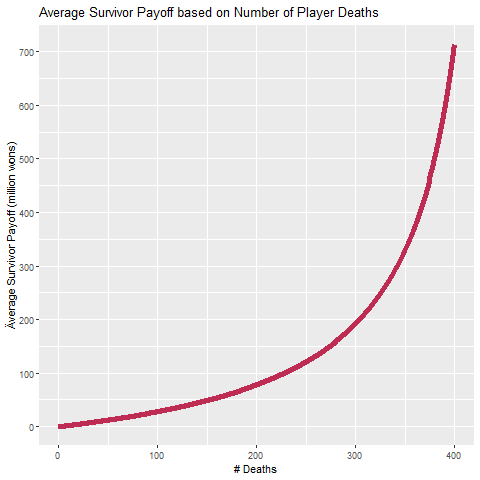
That’s quite the hockey stick shape if I ever saw one! But it shouldn’t come as too much of a surprise as both numerator and denominator favor many deaths: as the number of deaths increases, so does the piggy bank amount, but the number of survivor decreases, the hen taking the ratio we have something that really shoots up with a maximum of 45.5 billion wons!
Note 2: In the series, it is often said the single winner leaves with 45.6 billion wons, I’m guessing the organizers of the game might throw in an extra 100 million wons to the jackpot which corresponds to the ”value” of the player.
Note 3: Back to our conversions, the total jackpot of 45.6 billion wons is equivalent to approximately $31.5 million.
Now for a trickier question: in the series, the first post-challenge votes are all in favor of continuing to play extra challenges, why is that?
This is a much more subjective question, and of course each of the 456 players has their own rationale, debt, thresholds, risk aversions… But based on the game set-up we can take a stab at understanding how players approach an extra challenge.
Let’s first answer another question: if every player’s “value” is $100 million wons (value that gets added to the piggy bank if they die), how many deaths need to occur for the average payoff to be that same value?
Given the formula previously derived, we can easily see that if average payoff is equal to player value, then number of deaths / (456 - number of deaths) must be equal to 1, meaning there are as many deaths as survivors, and so exactly half the initial players died. 228 players!
What about if players want to leave with double their value, or triple, or multiply by 10? If we define f as the factor of how many multiples of their value survivors leave with, we have:
f = number of deaths / (456 - number of deaths) which w can flip to:
number of deaths = 456 * f / (f + 1)
So to double payoff, 304 deaths would be required which is only 76 more than the 228 that were required to get the player value as payoff!
And so the minimum number of deaths required to get multiples of the $100 million player value is:
And we can see the full visual here:
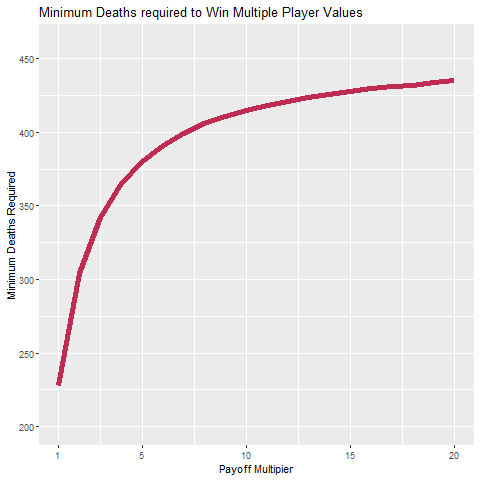
It takes fewer and fewer deaths to get significantly higher payoffs, which is of course another interpretation of the very first hockey stick figure we saw.
Here's an alternative ingographic-style view:

Back to our question, why do players keep voting for an extra challenge despite the risk lethality?
Based on our previous work, we can split the decision-making into two phases:
Phase 1
Players in the game usually have rather high debts, and payoffs are really horrible at the very beginning given how many players are still alive to divide up the piggy bank amount. In this phase payers need to continue to actually get something out of having risked their lives.
Phase 2
At some point, quite a few survivors could leave with a payoff sufficient to cover their debts, so the incentive to stay should decrease? But another phenomenon kicks in, the average payoff is starting to skyrocket. Every time a few extra players die, the average payoff starts multiplying! It is therefore likely that many players will start thinking along the lines of “I survived 342 other deaths which is a survival rate 25%, surely I can survive another 23 deaths of the remaining 114 players (survival rate of about 80%), and leave with quadruple the player value instead of just triple!”
The organizers of the games have masterfully set-up the payoff system to generate and combine these two psychological effects in order to ensure games would continue through many challenges to the greatest delight of the VIP watchers… and to all Netflix subscribers!


