Infographic: Fight for the Eastern Conference #1 Seed

All season-long, Indiana set the #1 seed as their objective. While the Pacers completely dominated the first half of the season, they crumbled after the All-Star break (at the same time that Miami and Oklahoma) letting San Antonio capture the overall seed.

But while the overall top seed slipped through their fingers, keeping their grasp on the #1 Eastern conference seed against Miami was a nail-bitting battle till the last few games of the season.

The following infographics show which team had the best winning percentage throughout the regular season. The line is blue when Indiana has the best percentage, red when Miami had it.

Overall season evolution:

Since the All-Star break:

From a 'Ganes Behind' perspective:

Best of the West or best of the rest?

The NBA finals are right around the corner. Only a handful of games are left to be played in this 2013-2014 season, and homecourt advantage is still a hard fought battle for the top teams.

Miami wants it to increase their odds of winning a third straight championship, Indiana wants it to turn the tables if (more like when) it meets Miami in the Eastern conference finals and avoid a game 7 in Miami like it did last year, San Antonio wants it for the exact same reason except it lost to Miami in game 7 of the finals, and OKC wants it in case it faces Miami in the finals (plus it could provide Kevin Durant with an additional edge on the MVP race against LeBron James).

So yes, everyone wants homecourt advantage, it's been proved over and over again (including in this blog) that there is a definitive advantage to playing 4 games instead of 3 at home in the best-of-7 format. But how key is it really? Does homecourt advantage really determine the NBA champions? Do other factors such as the conference you are in or the adversity faced in the first rounds play a part?

Following on the tradition of the past years, the West is clearly better than the East. Consider this: right now, the Phoenix Suns hold the eighth-best record in the West with 46 wins and 31 losses, and has the last seed for the playoffs. But only two teams have a better record than that in the East, Miami and Indiana. Stressing to hold the last playoff spot in one conference versus a comfortable third seed in the other? Talk about disparity!

But if you had to guess whether the next champ was going to be from the East or West what would you say? That the eastern team would have an easier road to the finals, less games, less fatigue than their western counterpart? Or does evolving in a hyper-competitive bracket strengthen you, in a what-doesn-t-beat-you-makes-you-stronger argument?

Does the overall strength conference have an impact? Does the team with the best regular season record (and hence homecourt advantage) necessarily win? Does the team with the easiest path to the finals have an advantage?

To investigate this I've looked at all championships since 1990 (24 Playoffs) and looked in each case at some key stats for the two teams battling for the Larry O'Brien trophy, among these:

• number of regular season wins
• regular season ranking
• sum of regular season wins for opponents encountered in the Playoffs
• sum of regular season ranking for opponents encountered in the Playoffs
• number of games played to reach the Finals
• sum of regular season wins for all other Playoffs teams in their respective conferences
• sum of regular season ranking for for all other Playoffs teams in their respective conferences
• ...

So for Miami in 2013, the data would look something like:

• 66 regular season wins
• NBA rank: 1
• played 16 games before reaching the Finals
• 132 playoff opponent regular season wins (Indiana: 49, Chicago: 45, Milwaukee: 38)
• 38.5 playoff opponent regular NBA ranking (Indiana: 8.5, Chicago: 12, Milwaukee: 18)
• 320 playoff conference regular season wins (Indiana: 49, New York: 54, Chicago: 45, Brooklyn: 49, Atlanta: 44, Milwaukee: 38, Boston: 41)
• 84.5 playoff opponent regular NBA ranking (Indiana: 8.5, New York: 7, Chicago: 12, Brooklyn: 8.5, Atlanta: 14 Milwaukee: 18, Boston: 16.5)
• ...

As for the Spurs who were the other 2013 finalists, they had a worse record, emerged from a tougher conference and met stronger opponents while needing surprisingly less games to reach the Finals:

• 58 regular season wins
• NBA rank: 3
• played 14 games before reaching the Finals
• 148 playoff opponent regular season wins (LA Lakers, Golden State, Memphis)
• 27.5 playoff opponent regular NBA ranking (LA Lakers, Golden State, Memphis)
• 366 playoff conference regular season wins (Memphis, Oklahoma, Golden State, Denver, Houston, LA Lakers, LA Clippers)
• 51 playoff opponent regular NBA ranking (Memphis, Oklahoma, Golden State, Denver, Houston, LA Lakers, LA Clippers)
• ...

I then ran various models (simple logistic regression, and lasso logistic regression) to see how these different metrics helped predict who would win the champion come the Finals.

The conclusions confirmed our intuition:

• having more regular season wins that your opponent in the Finals provides a big boost to your chance of winning (namely by securing homecourt advantage, but the exact number of games provided a much better fit than a simple homecourt advantage yes/no variable)
• there were indications that having a tougher path to reach the finals (more games, tougher opponents) slightly reduced the probability of winning the championship, but none of those effects were very significant

The effect from difference in regular season wins can be seen on the following graph, where we have compared two (almost) identical teams evolving in identical conferences. The only difference between the two teams is the number of wins they've had in the regular season, shown on the x-axis. The y-axis shows the probability of winning the championship.

A five-game differential in wins will translate with a 73% / 27% advantage to the team with the most wins. Only a one-game advantage translates into a 55% / 45% advantage.

The conference effect appears quite minimal, and home-court advantage appears to be key. If Indiana hates itself right now for having let the number 1 seed in the East slip through its fingers, it can always try to comfort itself with the fact that (unless a major San Antonio / Oklahoma / LA Clippers break down occurs over the remaining games of the season), the Western team making it to the Finals would have held homecourt advantage no matter what.

It should also be noted that a "bad" conference isn't synonym of easy opponents. Just look how Brooklyn seems to have the Heat's number this year, the way Golden State had Dallas' in 2007 when it beat the number 1 seed in the first round. All season long the Golden State Warriors were the only ones who could match up against Dallas really well.

UPDATE: as of yesterday, Indiana has reclaimed the top seed in the East, but the final argument can be applied to Miami just as well. Whichever of these teams makes it to the Finals will face a tough opponent.

Easy tips for Hollywood Producers 101: Cast Leonardo DiCaprio! (but cast him quick!)

My wife and I were thinking of going out to see "The Wolf of Wall Street" the other day. Why did this movie catch our eye more than the other twelve or such showing at our local movie theatre?

Had we heard great reviews about it? Nope. Had word-of-mouth finally reached us? Nope. Had we fallen prey to a cleverly engineered marketing campaign? Well yes and no.

Not owning a TV at home, so the least you could say is that our TV ad exposure was quite minimal. And as far as I can remember (although one could argue that this is exactly the purpose of sophisticated inception-style marketing) we din't see that many out-of-home ads nor hear any radio ones. Marketing was involved, but the genius of the marketers behind "The Wolf of Wall Street" was restricted to creating the poster, and not because of the monkey in a business suit nor the naked women, but simply by putting Leonardo DiCaprio right there. My wife and I's reasoning was simply that any movie with Leonardo had to be good.

Now don't go and write us off as Titanic groupies/junkies. I won't deny we both enjoyed that movie, but we don't have posters of him plastered all over our house. But here's the question we found ourselves asking: Can you name a bad movie with Leonardo in it? And harder yet: a bad recent movie with him in it?

Made you pause for a second there didn't it? Few people will argue against the fact that Leonardo is a very good actor and that his movies are generally pretty darn good. But are we being totally objective here? How does Leonardo's filmography compare to that of other big stars? The Marlon Brandos, Al Pacinos, De Niros, Brad Pitts...?

In order to compare actors' filmographies, I turned to my favorite database from IMDB. IMDB has a rather peculiar way of listing actors, directors, producers in its database, and I was unable to find a logic between the individual and the index in the database. But I did notice that all the big actors I wanted to compare Leonardo to had a low index (never above 400), so decided to pull data for all indices less than 1000. Now in the process I got some directors or actors with very few movies, so excluded from the analysis anybody have acted in less than 10 movies. The advantage of pulling this way was the fact that it provided a very wide range of diversity in gender, geography and time. So we have Fred Astaire, Marlene Dietrich, Louis de Funès, Elvis Presley...And to get an even broader picture, I added 30 young rising new stars to the mix. All in all, 826 actors to compare Leonardo to.

Going back to our original question of how good Leonardo is, I've looked at two simple metrics: ratio of movies with an IMDB rating greater than 7, and ratio of movies with an IMDB greater than 8. So how well did Leonardo do? The mean fraction across the actors was 22% for the 7+ rating (median 20%). Leonardo had... 55%! That's 16 out of his 29 movies! Only 15 actors have a higher score. Top of the list? Bette Davis, with 76 of her 91 movies (83.5% having a 7+ rating). The recently deceased Philip Seymour Hoffman also beat Leonardo with 31 out of 52 (59.6%). Fun fact, what male actor of all times has the best ratio here? You have to think out of the box for this one as he's more famous for directing than acting, yet makes an appearance in almost every one of his movies. That's right, Sir Alfred Hitchcock, has 28 of 36 movies (77.8%) rated higher than 7.

Name	Number of movies	Number of 7+ movies	Ratio of 7+ movies
Bette Davis	91	76	83.5%
Alfred Hitchcock	36	28	77.8%
François Truffaut	14	10	71.4%
Emma Watson	14	10	71.4%
Bruce Lee	25	16	64.0%
Terry Gilliam	16	10	62.5%
Andrew Garfield	13	8	61.5%
Alan Rickman	44	27	61.4%
Frank Oz	31	19	61.3%
Daniel Day-Lewis	20	12	60.0%

What about for movies rated higher than 8? Leonardo does even better according to this metric! The average actor has only 2.7% (median 1.7%) of movies with such a high rating. Leonardo has 5 out of 29, 17.2%! And only 8 actors do better with this metric. No more Bette Davis (plummets to 3.2%), but replaced by Grace Kelly (3 out of 11, 27.3%) who tops the chart. Sir Alfred is impressive once again with 9 out of 36 (25%).

Name	Number of movies	Number of 8+ movies	Ratio of 8+ movies
Grace Kelly	11	3	27.3%
Alfred Hitchcock	36	9	25.0%
Anthony Daniels	12	3	25.0%
Chris Hemsworth	12	3	25.0%
Terry Gilliam	16	3	18.8%
Elizabeth Berridge	11	2	18.2%
Elijah Wood	56	10	17.9%
Groucho Marx	23	4	17.4%
Leonardo DiCaprio	29	5	17.2%
Quentin Tarantino	24	4	16.7%

Now the big stars we mentioned earlier do pretty well, just not as good as Leonardo:

Name	Number of movies	Number of 7+ movies	Number of 8+ movies	Ratio of 7+ movies	Ratio of 8+ movies
Marlon Brando	40	18	4	45.0%	10.0%
Brad Pitt	48	23	6	47.9%	12.5%
Robert De Niro	91	32	8	35.2%	8.8%
Leonardo DiCaprio	29	16	5	55.2%	17.2%
Clint Eastwood	59	19	6	32.2%	10.2%
Morgan Freeman	69	24	7	34.8%	10.1%
Robert Downey Jr.	68	17	1	25.0%	1.5%

Another thing worth repeating to put these numbers in perspective: we are not comparing Leonardo to your "average" Hollywood actor. Because of the way IMDB has matched actors with indices, we are comparing Leonardo to some of the greatest of all times here!

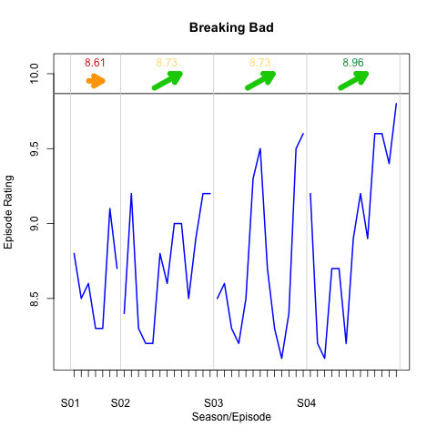
Remember how earlier one we mentioned that it was even harder to find a recent bad movie by Leonardo? Let's look at his movie ratings over time to confirm this impression:

Wow. With the exception of J.Edgar in 2011, every single one of his movies since 2002 (that's over this last decade !) has had a rating greater than 7! 12 movies!

Now one might argue that there is a virtuous circle here: the more you become a star, the easier it is to get scripts and parts for great movies and do the easier it becomes to continue being a super star. For each actor in my dataset, I ran a quick linear regression to see improvement of movie rating over time. Leonardo stands out here quite a bit too, for he is among the rare actors to have positive improvement. The "average" actor's movie lose 0.01 IMDB rating points per year, Leonardo gains 0.1 per year, putting him in the top 15 of the data set:

Name	Number of movies	Number of 8+ movies	Number of 7+ movies	Improvement
Taylor Kitsch	11	1	2	0.26
Rooney Mara	11	1	4	0.26
Justin Timberlake	18	0	3	0.23
Chloe Moretz	24	1	6	0.19
Bradley Cooper	26	0	7	0.18
Juliet Anderson	50	1	12	0.17
Mila Kunis	23	1	3	0.16
Chris Hemsworth	12	3	7	0.15
Tom Hardy	27	3	12	0.14
Andrew Garfield	13	0	8	0.12
Mia Wasikowska	21	0	9	0.12
Barbara Bain	14	1	2	0.11
George Clooney	38	1	15	0.11
Jason Bateman	32	2	9	0.11
Leonardo DiCaprio	29	5	16	0.10

What's quite surprising in the last table is that those topping the list in terms of year over year improvement are not the old well-established actors having great choice in scripts, but the new hot generation in Hollywood!

What happens to the megastars? Well let us look at the rating evolution of some of these stars:

Fred Astaire:

Marlon Brando:

Bette Davis:

It appears that they all go through some glory days. Remember Leonardo with his 12 years of 12 movies greater than 7 aside from J. Edgar? Well Bette Davis had 46 such movies, without any exceptions, over a span of 29 years! But not a great way to end a career... Same goes for Fred Astaire and Marlon Brando, started off doing well but end of careers are tough even for big stars, or might I say especially for big stars. Naturally, the hidden question is whether ratings of later movies go down because actors aren't as good as they were, or because good roles don't come as much, because they only get casted for grumpy grandparents in bad comedies. Correlation vs causation...

So back to Leonardo. He's still young, so the primary impulse my wife and I had of "Leonardo's in it so it's got to be good" was not completely irrational, but it might be in 5/10 years from now. Same goes for all the rising top stars. Cast them while they're hot, cause nothing is eternal in Hollywood.

Tuesday Oct 29 2013: Bulls at Miami, who will win?

The 2013-2014 NBA season kicks-off Tuesday October 29th and the spotlight will be the return of two of the injured megastars: the Bulls' Derrick Rose in Miami, and the Kobe Bryant's Lakers host the Clippers.

On this blog we love drama, we love high intensity games, but we also like tough questions. Such as: who will win those two games? And while we're at it, who will come out victorious of the other 1228 games of the season?

In this post I will present my efforts to predict the outcome of a game based on metrics related to the two opposing teams.

The data

The raw data consisted of all regular-season NBA games (no play-offs, no pre-season) since the 1999-2000 season. That’s right, we’re talking about 16774 games here. For each game I pulled information about the home team, the road team and who won the game.


The metrics

After pulling the raw data, the next step was to create all the metrics relate to the home and road team’s performance up until the game I want to predict the outcome of. Due to the important restructuring that can occur in a team over the off-season, each new season starts from scratch and no results carried over from one season to the next.

Simple Metrics
The simple metrics I pulled were essentially the home, road and total victory percentages for both the home team and the road team. Say the Dallas Mavericks, who have won 17 of their 25 home games and 12 of their 24 road games visit the Phoenix Suns who have won 12 of their 24 home games and 13 of their 24 road games, I would compute the following metrics:

• Dallas home win probability: 17 / 25 ~ 68.0%
• Dallas road win probability: 12 / 24 ~ 50.0%
• Dallas total win probability: 29 / 49 ~ 59.2%
• Phoenix home win probability: 12 / 24 ~ 50.0%
• Phoenix road win probability: 13 / 24 ~ 54.2%
• Phoenix total win probability: 25 / 48 ~ 52.1%

Discounted simple metrics
However, these statistics seemed a little too simplistic. A lot can happen in the course of a season. Stars can get injured or return from a long injury. A new team might struggle at first to play with each other before really hitting their stride. So I included some new metrics which have some time discounting. A win early in the season shouldn’t weigh as heavily as one in the previous game. In the non-discounted world we kept track, for home games and road games separately, of the number of wins and number of losses, incrementing one or the other by 1 depending on whether the team won or lost. We do exactly the same here with a discount factor:

new_winning_performance = discount_factor * old_winning_performance + new_game_result

new_game_result is 1 if they won the game, 0 if they lost.

When setting the discount factor to 1 (no discounting), we are actually counting the number of wins and are back in the simple metrics framework.

To view the impact of discounting, let us walk through an example:
Let’s assume a team won it’s first 3 games then lost the following 3, and let us apply a discount factor of 0.9.

• After winning the first game, the team’s performance is 1 (0 * 0.9 + 1)
• After winning the second game, the team’s performance is 1.9 (1 * 0.9 + 1)
• After winning the third game, the team’s performance is 2.71 (1.9 * 0.9 + 1)
• After losing the fourth game, the team’s performance is 2.44 (2.71 * 0.9 + 0)
• After losing the fifth game, the team’s performance is 2.20 (2.44 * 0.9 + 0)
• After losing the sixth game, the team’s performance is 1.98 (2.20 * 0.9 + 0)

But now consider a team who lost their first three games before winning the next three:

• After losing the first game, the team’s performance is 0 (0 * 0.9 + 0)
• After losing the second game, the team’s performance is 0 (0 * 0.9 + 0)
• After losing the third game, the team’s performance is 0 (0 * 0.9 + 0)
• After winning the fourth game, the team’s performance is 1 (0 * 0.9 + 1)
• After winning the fifth game, the team’s performance is 1.9 (1 * 0.9 + 1)
• After winning the sixth game, the team’s performance is 2.71 (1.9 * 0.9 + 1)

Although both teams are 3-3, the sequence of wins/losses now matters. A team might start winning more if a big star is returning after an injury of due to a coach change or some other reason so our metrics should reflect important trend changes such as those. Unsure of what the discounting factor should be, I computed the metrics for various values.

Discounted opponent-adjusted metrics
A third type of metric I explored was one where the strength of the opponent is incorporated to compute a team’s current performance. In the above calculations, a win was counted as 1 and a loss as 0, no matter the opponent. But why should that be? Just like in chess with the ELO algorithm, couldn’t we give more credit to a team beating a really tough opponent (like the Bulls snapping the Heat’s 27 consecutive wins), and be harsher when losing to a really weak team?
These new metrics were computed the same way as previously (with a discounting factor) but using the opponent’s performance instead of 0/1.

Let’s look at an example. The Thunder are playing at home against the Kings. The Thunder (pretty good team) have a current home win performance of 5.7 and a current home loss performance of 2.3. This leads to a “home win percentage” of 5.7 / (5.7 + 2.3) = 71%. The Kings (pretty bad team) have a current road win performance of 1.9 and a current road loss performance of 6.1. This leads to a “road win percentage” of 1.9 / (1.9 + 6.1) = 24%.

If the Thunder win:

• The Thunder’s home win performance is now: 0.9 * 5.7 + 0.24 = 5.37
• The King’s road loss performance is now: 0.9 * 6.1 + (1 - 0.71) = 5.78

If the Thunder lose:

• The Thunder’s home loss performance is now: 0.9 * 2.3 + (1 - 0.24) = 2.83
• The King’s road loss performance is now: 0.9 * 1.9 + 0.71 = 2.42

If you win, you get credit based off of your opponent’s win percentage. If you lose, you get penalized according to your opponent’s losing percentage (hence the 1- in the above formulas). The worst teams hurt you most if you lose to them.
As seen from the example between a very good team and a very bad one, winning does not guarantee that your win performance will increase and losing does not guarantee your losing performance will increase. The purpose is not to have a strictly increasing function if you win, it is to get, at a given point in time, an up-to-date indicator of a team’s home and road performance.


The models

For all the models, the training data was all games except those of the most recent 2012-2103 season which we will use to benchmark our models.

Very simple models were first used: how about always picking the home team to win? Or the team with the best record? Or compare the home team’s home percentage to the road team’s road percentage?

I then looked into logistic models in an attempt to link all the above-mentioned metrics to our outcome of interest: “did the home team win the game?”. Logistic models are commonly used to look at binomial 0/1 outcomes.

I then looked into machine learning methods, starting with Classification and regression trees (CART). Without going into the details, a decision tree will try to link the regressor variables to the outcome variable by a succession of if/else statements. For instance, I might have tracked over a two week vacation period whether my children decided to play outside or not in the afternoon, and also kept note of the weather conditions (sky, temperature, humidity,...). The resulting tree might look something like:

If it rains without wind tomorrow, I would therefore expect them to be outside again!

Finally, I also used random forest models. For those not familiar with random forests, the statistical joke behind it is that it is simply composed of a whole bunch of decision trees. Multiple trees like the one above are “grown”. To make a prediction for a set of values (rain, no wind), I would look at the outcome predicted by each tree (play, play, no play, play….) and pick the most frequent prediction.

The results

As mentioned previously, the models established were then put to the test on the 2012-2013 NBA season.

As most of the models outlines above use metrics that require some historical data, I can’t predict the first game of the season not having any observations for past games for the two teams (yes, I do realize that the title of the post was a little misleading :-) ). I only included games for which I had at least 10 observations of home games for the home team and 10 road games for the road team.

Home team
Let’s start with the very naive approach of always going for the home team. If you had used this approach in 2013, you would have correctly guessed 60.9% of all games.

Best overall percentage
How about going with the team with the best absolute record? We get a bump to 66.3% of all games correctly predicted in 2013.

Home percentage VS Road percentage
How about comparing the home team’s home percentage with the road team’s road percentage? 65.3% of games are correctly guessed this way. Quite surprisingly, this method provides a worse result than simply comparing overall records.

Logistic regressions
Many different models were tested here but I won’t detail each. Correct guesses range from 61.0% to 66.6%. The best performing model was the simplest one which only included the intercept and the overall winning percentage for the home team and the road team. The inclusion of the intercept explains the minor improvement to the 66.3% observed in the “Best overall percentage” section.
Very surprisingly, deriving sophisticated metrics discounting old performances in order to get more accurate readings on a team’s performance did not prove to be predictive.

Decision tree
Results with a decision tree was in the neighborhood of the logistic regression models, with a value of 65.8%.

Interestingly, the final model only looks at two variables and splits: whether the home team's home performance percentage (adjusted with a discounting factor of 0.5) is greater than 0.5 or not, and whether the road team's performance incorporating opponent strength (discounting factor of 1, so no discounting actually) is greater than 0.25 or not.

Random Forests
All our hopes reside in the Random Forests to obtain a significant improvement in predictive power. Unfortunately we obtain a 66.2% value, right where we were with the decision tree, the regression model and more shamefully the model comparing the two teams overall Win-Loss record!
When looking at which variables were most important, home team and road team overall percentages came up in the first two positions.


Conclusions

The results are slightly disappointing from a statistical point of view. From the simplest to the most advanced techniques, none are able to break the 70% threshold of correct predictions. I will want to revisit the analyses and try to break the bar. It is rather surprising to see how overall standings matter compared to metrics that are more time sensitive. The idea that the first few games of the season matter to predict the last few games of the season is a great insight. This can be interpreted by the fact that good teams will eventually lose a few consecutive games in a row, even against bad teams, but that should not be taken too seriously. Same with bad teams winning a few games against good teams, they remain bad teams intrinsically.

From an NBA fan perspective, the results are beautiful. It shows you why this game is so addictive and generates so much emotion and tension. Even when great teams face terrible opponents, no win is guaranteed. Upsets are extremely common and every game can potentially become one for the ages!

Boston: City of Champions

This is what I saw the other day at the Boston Airport (minus a hundred other people taking their shoes off and laptops out of carry-ons):

All the championships won by a Boston team (Celtics, Bruins, Patriots, Red Sox) have their banner hanging from the ceiling right before security screening. My daughter noticed the banners too and asked if they were ordered by color. I replied that they were actually ordered by date and when the championship was won.

But taking a second look at the ordered banners showed that her interpretation was not very far off the mark.

5 red banners, 3 yellow, 11 green, 2 yellow, 5 green, 3 blue, 2 red, 1 green, 1 yellow... The same colors seem to be close to each other (with some slight variation depending on the ordering of the third Patriot Superbowl championship and Red Sox title). So the natural question is whether any conclusions can be drawn from the fact that the colors seemed to be grouped together?

It could very well be that this is all purely coincidental: with only four teams capable of winning championships, you would expect at some point the same team to win two titles without one of the other three winning in between. But would the groupings be so obvious? A hypothesis would be that every so often, one of the teams will dominate its sport and that for a certain period of time will win way more than the other three Boston teams. When a team wins a given year, it has a much greater probability of winning the next than on a random year. So color clusters are actually proxys for team dominance during a certain era.


First approach

To determine which of the two reasoning is most likely, I ran a few simulations. By a few I mean a million. I considered 17 Celtics championships, 7 Red Sox championships, 6 Bruins championships and 3 Patriots championships, then randomly sampled without replacement. Our measurement of clustering is simply the number of clusters observed. The minimum number is 4 when all teams win all their titles without interruption (17 green, 7 red, 6 yellow and 3 blue, or 6 yellow, 3 blue, 17 green and 7 red, or...). The max is 33 when teams keep interrupting each other:
G-Y-G-Y-G-Y-G-Y-G-Y-G-Y-G-B-G-B-G-B-G-R-G-R-G-R-G-R-G-R-G-R-G-R-G.

In Boston history we have 9 transitions which is definitely on the low side. The histogram for a million simulations yields:

The average and median number of clusters was greater than 22. Not only is our observation of 9 (red vertical line) much lower, but not a single of our 1000000 simulation yielded a value less than 10! Talk about p-value!


Second Approach

We definitely simplified the true dynamics on championship winning by considering our urn of championships from which we picked. A second approach would be to look year by year at the probability of a team winning a championship.

Based on our observations of the last 114 years (assuming a start date in 1900) the Celtics won 17 times, the Red Sox 7 times, the Bruins 6 times and the Patriots 3 times. We can therefore use these empirical probabilities to generate other what-if scenarios where each year the probability of any team winning is independent of the past (no team dominance).
With this simple approach I only consider that a single team can win in any given year. Starting in 1900, I flip a very biased 5 sided-coin where Celtics come up with probability 17/114, Red Sox 7/114, Bruins 6/114, Patriots 3/114 and Nobody with 81/114. And then look again at how many clusters are obtained.

In the first approach we sampled without replacement from an urn with 33 championships. However in our new approach we could get no championship at all every single year or a championship every single year! We can't just compare the number of clusters, but should instead look at cluster average: # transitions / # championships. In real life the ratio is 8/33  ~ 0.2424. In our new 1000000 sample we were able to generate a few cases that out-performed real life where 8 transitions were also observed but with 34 and even 36 championships. Some very low values of averages were observed when the number of championships won was almost half (4 transitions and 19 championships, this was huge Celtics dominance!). That being said, only 39 out of 1000000 simulations yielded an equivalent or better ratio. Here's a plot of the distribution of cluster-to-championship ratio, with the red line indicating what we observed in Boston:

So no matter how simple our approaches, we have definitely put forward some evidence of sports dominance by Boston's teams (and luckily for our analysis, Boston's teams did not dominated at the same time too often or that would have created some high frequency alternating between the two teams, thus breaking our clustering metric).

I don't believe my three-year old grasped all the subtleties involved here, but I definitely hope all those bright colors will get here interested in stats!

Visualizing the quality of a TV series

I love TV series. Like many people, my first addiction was Friends. Only 20 minutes, 4 jokes-a-minute, it was easy to fit in your schedule.

Then came the TV series revolution, with more sophisticated scripts, each episode becoming less of an independent unit but one of the many building blocks in the narration of ever increasing complex plots. Skipping episodes was no longer an option, even more so given the cliffhanger of the last episode.
The first such series I remember were 24 and Lost.

I'm not going to list all my favorite shows, nor try to compare them or do any advanced analyses. I just wanted to share some visuals I created allowing quick summarization of the quality of a series, episode after episode, season after season.

Here is the visual for Friends:

The blue line displays the IMDB rating of the episodes within each season - notice the break between seasons and the gray vertical bars delimiting seasons. There is a lot of data represented, so I've added some summary stats at the very top of each season:

• the number at the very top is the average of the IMDB rating for all the episodes of the season. The color on a red-green scale compares the seasons to each other: the seasons with highest averages are green, those with worst ratings are red.
• the arrow under the season average represents the evolution of ratings within the season: if episodes tend to get better and better the arrow will point upwards and be green, if they get worse the arrow will point downwards and be red. If the ratings remain approximately average over the season a horizontal orange arrow is displayed.

Revisiting the Friends visual, we observe spectacular consistency in ratings over the ten-year period. The summaries on top allow us to see through the noise, and that seasons 8 and 9 were among the worst in average episode rating as well as the only two that got worse over the season. But the tenth and final season was the highest-rated one, and had a strong positive trend until the series finale.

Although not a huge fan, I had to look at the Simpsons' incredible run. The visual highlights the surprising drop and plateau of the season average starting around the ninth season.

Now looking at some of my favorite series:

I have to agree here that the first seasons of 24 were the best. I also love the way ratings evolve in the final season, when people had very low expectations and thought it would be the same old jack-bauer-aka-superman-prevents-nuclear-attacks-every-thirty-minutes but soon realized this was Jack Bauer on a revenge rampage without any rules.

Breaking Bad is the perfect example of the TV series that keeps getting better, throughout the seasons and throughout the years. Can't wait for the second half of the fifth season!

The last few seasons of Dexter aren't rated as high as the first ones, but ratings remain high.

I loved the first season of Prison Break but clearly it should have been a one-season series, you jsut couldn't top the suspense and originality.

Game of Thrones started really high but just kept getting better à-la-breaking-bad. The seesaw effect in the third season is rather impressive!

Hollywood's lack of originality: "Let's make a sequel!" (Part 3, yes I realize the irony)

As indicated by the title, this is part 2 of the analysis of movie sequels.
In the first post I described the IMDB data used for the analysis and shared some preliminary statistics on the distribution of number of movie installments in movie series.
In part 2 I focused on comparing IMDB ratings for the original movie and its sequel.

This post looks at series with 3 or more installments.

The sequel has a sequel!!!

Looking at multiple installments is a little tricky. Can I compare the average IMDB rating change between installments 1 and 2 with the change between installments 2 and 3? Probably, but only if I look at the same sample. Let me explain myself. To compute the change between installments 1 and 2 I might have 1000 series to look at (2000 movies then). But when looking at the change between 2 and 3, my sample will be smaller (I will no longer have all the series that only had two installments). Is that so much of an issue? It could be if there is what is called a "lurking third variable". Perhaps moviemakers only make a third installment when the second installment wasn't too bad, so series with only two installments could be biased in the sense that they are the ones where the second installment did really terrible and so no third installment was made. So if we really want to compare the drop-off between 1 and 2 with the drop-off (I am assuming it is another drop-off!) between 2 and 3, we should restrict the analysis to only series with at least three installments.

So there are a couple of things we might want to look at:
1) average change between installments 1 and 2 for all movies that have 2 and only 2 installments
2) average change between installments 1 and 2 for all movies that have 3+ installments
3) average change between installments 2 and 3 for all movies that have 3+ installments

Comparing 1) and 2) will give us an idea whether third installments are favored for series where second installments didn't do too badly. Comparing 2) and 3) will allow us to compare the 1 -> 2 and 2 -> 3 effects.

Here are the results:

Series length	Sample Size	From Installment ...	To installment ...	IMDB Rating Difference
All series	606	1	2	-0.87
Exactly 2	410	1	2	-0.92
3 or more	196	1	2	-0.78
3 or more	196	2	3	-0.33

So it does seem that series with exactly 2 installments had a larger 1 to 2 installment drop-off (-0.92) than those with 3 or more installments (-0.78), however another (unpaired) t-test revealed that the difference was not significant. Budget and revenue are probably more important factors than IMDB ratings taken into account at Hollywood before deciding whether to make a third movie, but I suspect there is still some correlation between rating and revenue (no worries a future post will address this!).

Another interesting finding is that the drop-off from 2 to 3 is much smaller than from 1 to 2. This can make sense: 
1) First of all, an IMDB rating can only go so low, you can't keep losing a full point rating everytime.
2) It is safe to assume the original movie was seen by a rather diverse crowd, whereas the second might have been seen only by the first movie's fan base, and very likely that those were about the same as those who saw the third. In other words, a much bigger overlap is to be expected between those who saw the second and third as opposed to first and second, which translates into more similar ratings.

More than 3?

For more than three installments, the sample starts to shrink quite rapidly, which is why I went for a more visual approach. I normalized all first installments to a score of 100 in order to track the evolution of all subsequent installments. This graph will allow us to shed some light on some hypotheses from the previous section: ratings go down but at a slower pace and tend might eventually converge with the same hard-core fan base rating the movies.

A slightly more confusing plot where trends are harder to establish but which nonetheless conveys both the initial rating drop-off as well as the sharp decrease in series length is the spaghetti-plot, where each line represents the evolution of a given series rating installment after installment.

From the previous two graphs, it appears that the decrease we observed over the first few installments continues until the fourth installment which is typically a series all-time low, with installments 5 and 6 usually bouncing surprisingly back. However, as shown in the spaghetti plot, the sample size is severely reduced and it would be dangerous to draw any strong conclusions.

It also seemed that quite a few series ended on surprisingly good ratings, sometimes the best or second best after the first installment:

• The Rocky series was strictly decreasing from the start: 8.0, 6.9, 6.3, 6.2, 4.7 but finished with 7.2
• The Rambo series had a similar pattern: 7.5, 6.0, 5.2, and...  7.1!
• The Harry Potter series has ratings grouped between 7.2 and 7.6 for the first 7 installments but the eight and final finished at 8.1

Could it be that for these series a real effort was made to finish on a strong note? Stallone probably put more thought into the script waiting 16 years for the last Rocky whereas the first 5 came within an average of 3 to 4 years apart from each other. Same for Rambo within a 20 year lapse compared to the three year gaps for the first movies.

Also, in the cases mentioned above, the last installment was usually declared as such, in which case also ratings might be higher from fans saddened to witness the final installment.

Closing thought

What have we learned? The primary conclusion is that the common belief that sequels do worse than the original is definitely valid. Although not proven here, the most likely explanation is that Hollywood doesn't care about making terrible movies as long as they generate a profit but more importantly (since good movies are more likely to generate greater profits than terrible movies, a priori) they want as little risk as possible involved. A guaranteed million dollar profit is better than a 50/50 chance of generating either three million or losing a million.