The Capitalistic Whirlpool (or "why there is mathematically no hope the players will vote to stop playing Squid Game")

Squid Games season 2 was a highly anticipated new season, and it certainly did not disappoint! Before I write another sentence, please be mindful some very high level spoilers will here be revealed, rest assured, nothing along the lines of “Player XYZ dies in episode 4”, but we will be digging into some of the rules of the game, so if you’re planning on watching Squid Games some day and want to be 100% surprised by it, please don’t read any further!

As a quick recap and to accurately define our variables, the high level rules in Squid Game are as follows:

• 456 players are in the overall game

• The game is split into individual challenges

• Every time a player dies in a challenge, 100 million wons are added to a common piggy bank ( from here on out we will refer to these 100 million wons as ‘player value’)

• After each challenge, players can vote on whether to continue for another challenge, or stop there and split the money accumulated in the piggy bank equally amongst the survivors

For example, if 10 players die in the first challenge, then 1 billion wons (10 times 100 million wons) will be added to the piggy bank, and if the remaining 446 players (456 original players minus the 10 dead) decide to stop after that first challenge, each will leave with 100 million * 10 / 446 = 2.24 million wons. 

Note 1: it is sometimes difficult to grasp these very large amounts in Korean wons. 1 won being equal to just 0.00069 dollars, each player’s value of 100 million wons is equivalent to about $69,000.

Which brings us to today’s first question: what does the curve for payoff-per-survivor look like as a function of the number of players having died so far?  

We’ve seen what one data point on that curve looks like for 10 deaths, but we can easily generalize:

Average survivor payoff = (money in piggy bank) / (number of survivors)

                                       = $100 millions * number of deaths / (456 - number of deaths)

And the curve looks something like (y-axis in billion wons):

We can zoom in on the first 0-400 deaths (y axis in million wons):

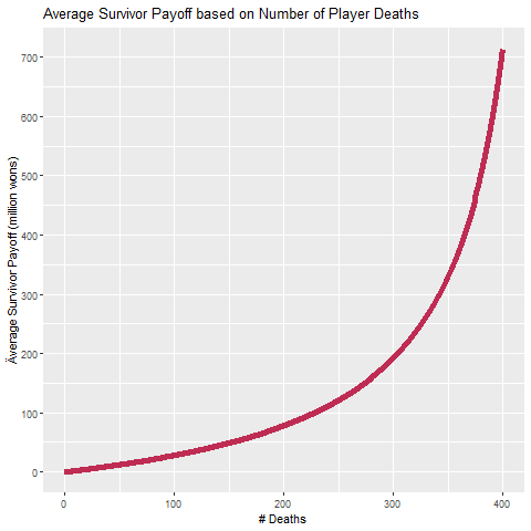
That’s quite the hockey stick shape if I ever saw one! But it shouldn’t come as too much of a surprise as both numerator and denominator favor many deaths: as the number of deaths increases, so does the piggy bank amount, but the number of survivor decreases, the hen taking the ratio we have something that really shoots up with a maximum of 45.5 billion wons!

Note 2: In the series, it is often said the single winner leaves with 45.6 billion wons, I’m guessing the organizers of the game might throw in an extra 100 million wons to the jackpot which corresponds to the ”value” of the player.

Note 3:  Back to our conversions, the total jackpot of 45.6 billion wons is equivalent to approximately $31.5 million.

Now for a trickier question: in the series, the first post-challenge votes are all in favor of continuing to play extra challenges, why is that?

This is a much more subjective question, and of course each of the 456 players has their own rationale, debt, thresholds, risk aversions… But based on the game set-up we can take a stab at understanding how players approach an extra challenge.

Let’s first answer another question: if every player’s “value” is $100 million wons (value that gets added to the piggy bank if they die), how many deaths need to occur for the average payoff to be that same value?

Given the formula previously derived, we can easily see that if average payoff is equal to player value, then number of deaths / (456 - number of deaths) must be equal to 1, meaning there are as many deaths as survivors, and so exactly half the initial players died. 228 players!

What about if players want to leave with double their value, or triple, or multiply by 10? If we define f as the factor of how many multiples of their value survivors leave with, we have:

f = number of deaths / (456 - number of deaths) which w can flip to:

number of deaths = 456 * f / (f + 1)

So to double payoff, 304 deaths would be required which is only 76 more than the 228 that were required to get the player value as payoff!

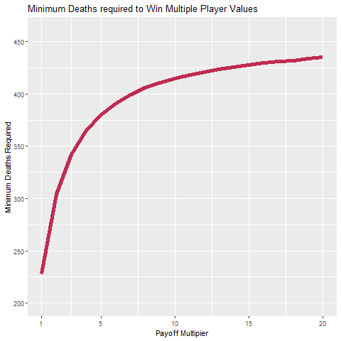
And so the minimum number of deaths required to get multiples of the $100 million player value is:

Factor	Survivor Payoff (million wons)	Minimum number of deaths	Incremental deaths required
1	100	228	228
2	200	304	76
3	300	342	38
4	400	365	23
5	500	380	15
10	1000	415	35

And we can see the full visual here:   

It takes fewer and fewer deaths to get significantly higher payoffs, which is of course another interpretation of the very first hockey stick figure we saw.

Here's an alternative ingographic-style view:

Back to our question, why do players keep voting for an extra challenge despite the risk lethality?

Based on our previous work, we can split the decision-making into two phases:

Phase 1

Players in the game usually have rather high debts, and payoffs are really horrible at the very beginning given how many players are still alive to divide up the piggy bank amount. In this phase payers need to continue to actually get something out of having risked their lives. 

Phase 2

At some point, quite a few survivors could leave with a payoff sufficient to cover their debts, so the incentive to stay should decrease? But another phenomenon kicks in, the average payoff is starting to skyrocket. Every time a few extra players die, the average payoff starts multiplying! It is therefore likely that many players will start thinking along the lines of “I survived 342 other deaths which is a survival rate 25%, surely I can survive another 23 deaths of the remaining 114 players (survival rate of about 80%), and leave with quadruple the player value instead of just triple!”

The organizers of the games have masterfully set-up the payoff system to generate and combine these two psychological effects in order to ensure games would continue through many challenges to the greatest delight of the VIP watchers… and to all Netflix subscribers!

Solving Mathematical Challenges with R: #3 Sum of all grids

Welcome to our third challenge!

You can find more details on where these challenges come from and how/why we will be approaching them in the original posting.

Challenge #3

The original link to the challenge (in French) can be found here. The idea is to consider an empty three-by-three grid, and then place two 1s in any two of the nine cells:

The grid is the completed as follows:

• pick any empty cell
• fill it as the sum of all its neighbors (diagonals as well)

I've here detailed an example, the new cell is indicated at each step in red:

The challenge is now to find a way to complete the grid in such a manner as to obtain the greatest value in a cell. In the previous example, the maximum obtained was 30, can we beat it?

Power grid

I strongly encourage you to try out a few grids before continuing to read. Any guesses as to what the greatest obtainable value is?

As you try it out, you might realize that the middle cell is rather crucial, as it can contribute its value to every other cell, thus offering the following dilemma:

• fill it too soon and it will be filled with a small value
• fill it too late and it will not be able to distribute its value to a sufficient number of other cells

Gotta try them all!
In the spirit of our previous posts, let's try all possibilities and perform an exhaustive search.
The first thing we need to ask ourselves is the number of possible ways of filling up the square, and then generating all those combinations in R.
Ignoring how the cells are filled up, there are 9 possibilities to fill up the first cell (with a 1), 8 possibilities for the second (also a 1), 7 for the third (with the rule)... and 1 for the ninth final cell. Which amounts to 9*8*7*...*1 = 9! = 362880, piece of cake for R to handle.

Generating permutations
So we want to generate all these possibilities which are actually permutations of numbers 1 through 9, where each number corresponds to a cell. {7,1,5,2,4,9,3,8,6} would mean filling up cells 7 and 1 first with a 1, then filling up cell #5, then #2 and do on.
A naive method would be to use expand.grid() once again for all digits one through 9, which would also give unacceptable orders such as {7,1,5,2,1,3,6,8,9} because cell #1 is filled twice at different times! We could easily filter those out by checking if we have 9 unique values. But this would amount to generating all 9*9*9..*9=9^9>=387 million combinations and narrow down to just the 362K of interest. That seems like a lot of wasted resources and time!

Instead, I approached the problem from a recursive perspective (R does have a package combinat that does this type of work, but here and in general in all the posts I will try to only use basic R):

• If I only have one value a, there is only a single permutation:{a}
• If I only have two values a and b, I fix one of the values and look at all permutations I have of the left-over value, then append the value that was fixed:
  - fix a, all permutations of b are {b}, then append the a: {b,a}
  - fix b, all permutations of a are {a}, then append the b: {a,b}
  - the result is {a,b} and {b,a}
• with three values, repeat the process now that we know all permutations of 2 values:
  - fix a, all permutations of b,c are {b,c} and {c,b}, then append the a: {b,c,a}, {c,b,a}
  - fix b, all permutations of a,c are {a,c} and {c,a}, then append the b: {a,c,b}, {c,a,b}
  - fix c, all permutations of a,b are {a,b} and {b,a}, then append the c: {a,b,c}, {b,a,c}

In R:
SmartPermutation <- function(v) {
  if (length(v) == 1) {
    return(as.data.table(v))
  } else {
    out <- rbindlist(lapply(v, function(e) {
      tmp <- SmartPermutation(setdiff(v, e))
      tmp[[ncol(tmp) + 1]] <- e
      return(tmp)
    }))
    return(out)
  }
}

Computing the score

The next and final step is to fill out the grid for each possible permutation.

This is done by defining a static mapping between cell ID and its neighbors:

We then go through each permutation, fill out a virtual grid (in our case it's not a 3-by-3 but a vector, which doesn't change anything as long as the relationships between neighbors is maintained) and track maximum value.

Neighbors <- function(i) {
  neighbor.list <-
    list(c(2, 4, 5), c(1, 3, 4, 5, 6), c(2, 5, 6),
         c(1, 2, 5, 7, 8), c(1, 2, 3, 4, 6, 7, 8, 9), c(2, 3, 5, 8, 9),
         c(4, 5, 8), c(4, 5, 6, 7, 9), c(5, 6, 8))
  return(neighbor.list[[i]])
}

CompleteGrid <- function(row) {
  grid <- rep(0, 9)
  grid[row[1 : 2]] <- 1
  for (i in 3 : 9) {
    grid[row[i]] <- sum(grid[Neighbors(row[i])])
  }
  return(max(grid))
}

Final answer
Based on our exhaustive search, we were able to identify the following solution yielding a max value of...57!

Little bonus #1: Distribution
The natural question is around the distribution of values? Were you also stuck around a max value in the forties? 57 seems really far off, but the distribution graph indicates that reaching values in the forties is already pretty good!

Little bonus #2: Middle cell
Do you remember our original trade-off dilemma? How early should the middle cell be filled out? In the optimal solution we see it was filled out exactly halfway through the grid.
To explore further, I also kept track for each permutation when the middle cell was filled out and what its filled value was. The optimal solution is shown in green, the middle cell being filled out in 5th position with a seven.

And a similar plot of overall max value against position in which the middle cell was filled:

It clearly illustrates the dilemma of filling neither too late nor too early: some very high scores can be obtained when the middle cell is filled as 4th or 6th cell, but absolute max of 57 will only be achieved when it is filled in 5th. Filling it in the first or last three positions will only guarantee a max of 40.

Solving Mathematical Challenges with R: #2 Slicing Cubes

Welcome to the second challenge!
You can find more details on where these challenges come from and how/why we will be approaching them in the original posting.

Challenge #2

The original link to the challenge (in French) can be found here. It's easy to understand but non-trivial to wrap one's head around...
Consider a nice perfect cube. So far so good. Consider slicing this cube with a Samurai sword in one swift straight cut. Now take a look at the 2D shape created by the cut on the cube. What types of shape can it be? We are primarily interested in whether or not it can be a regular polygon (equilateral triangle, square, regular pentagon, regular hexagon...).

Starting simple: Square

Let's look at some of the simpler shapes. Ironically, the simplest solution is not the equilateral triangle but the square. Can the slice lead to a square? After a few virtual cuts in your mind, you will have noticed that if the cut is parallel to any side, the shape of the slice will be a square!

Equilateral triangle

A little trickier, but a few additional virtual slicing and dicing should reveal the answer. Select a corner of the cube (technically, a vertex). Then move away from that corner along the three edges that make up the corner by an equal amount. The dimensional plane going through those three points (there is one and only one such plane: in 2D there is one and only one line going through two distinct points, in 3D there is one and only one plane going through three distinct points) will lead to an equilateral triangle:

The proof is straightforward: because we moved away from the corner by a constant value in all three directions, the three sides of the triangle are all equal to each other (square root of twice the square of the constant value, thanks Pythagoras!).

3-D Plotting in R

Before continuing, one question you might have is how the previous visuals were generated. Let's remind ourselves these posts are not as much about solving the challenge but also about expanding our R skills!
There are multiple functions and packages, but I was aiming for simplicity. I used the lattice package which has the benefit of containing lots of other functions so probably a good idea to have it installed once and for all, not only for the purpose of this challenge. Within that package, wireframe() is the function of interest.
The simplest way to use it is to provide a matrix where the value of the i-th row and j-th column is the altitude at the i-th index on the x-axis and j-th index on the y-axis. This assumes that all points on the x-axis and y-axis are equidistant. Alternatively, you can create a data.frame (say df) with columns for the x, y and z values. Then simply call wireframe(z ~ x + y, data = df) and you're good! There are multiple parameters for the shading, viewpoint angle and so forth...
Let's just run the basic example from the help file using the pre-loaded volcano dataset which is a 87 * 61 matrix:
wireframe(volcano, shade = TRUE, aspect = c(61/87, 0.4), light.source = c(10, 0, 10))

The z-axis label was slightly truncated, but aside from that it's a pretty nice plot for one-line of code!

Back to our cube
We solved the 3 and 4 sided regular polygons, but what about, 5, 6, 7...
We could continue playing around, but visualizing these slices is pretty tricky you'll have to admit!
So how can R help? Well how about generating a whole bunch of planes and looking at the type of slices we obtain?

To do that, a tiny little bit of algebra first. The general equation of a 2D plane in 3D is:
z = a + b * x + c * y
[well the purists might disagree and they would be correct, how about the vertical plane satisfying x = 0? It's not covered by the previous equation]
However the planes not covered are all the x = constants and y = constants which either don't slice the cube, or slice parallel to certain sides of the cube which we showed leads to squares!

So now, all we need to do is generate a whole bunch of a, b and c values, and see where the resulting plane intersects the cube.

Step 1: Edge intercepts
Again a little algebra, but there are 12 edges the plane could potentially intercept:

• the four vertical edges, parallel to the z axis, corresponding to {x=0 and y=0}, {x=0 and y=1}, {x=1 and y =0} and {x=1 and y=1}
• the four edges parallel to the x-axis
• the four edges parallel to the y-axis

In each case we can fit two of three values of x, y and z into the equation of the plane and get the third value.
Example: for x=0 and y=1, the equation becomes z = a + c. So the plane intercepts that edge at {x=0, y=1,z=a+c}.

So we end up with 12 points.

Step 2: Valid edge intercepts
For an edge to be valid, the third computed coordinate should be between 0 and 1. In our previous example, {x=0, y=1,z=a+c} is part of the cube if and only if 0 <= a + c <= 1.
We then filter to only keep the valid intercepts.

Step 3: Resulting figure?
Once we know how the cube was intercepted, we need to determine if we luckily stumbled across a special polygon!
To do that, I did the following:

• compute all distances between intercepts (only once so as not to compute everything twice, needless to have both A --> B and B --> A)
• keep the smallest value(s)
• count the number of occurrences of that smallest value
• if the number of occurrences is equal to the number of intercepts, we have ourselves a winner!

Illustration

Consider the square ABCD of side 1. I would compute all 6 possible distances:

• A --> B: 1
• A --> C: sqrt(2)
• A --> D: 1
• B --> C: 1
• B --> D: sqrt(2)
• C --> D: 1

I keep the minimal values:

• A --> B: 1
• A --> D: 1
• B --> C: 1
• C --> D: 1

I have four matches of the minimal value, same as number of points, I have a square!

The reason this works is that a regular polygon is convex, so the sides are the smallest distances between points (convex polygons on the left, concave on the right):

Running through a whole bunch of values for a, b and c (remember expand.grid() from the first challenge?) I got the following results for number of identified regular polygons based on number of intercepts:

#Intercepts   Not Regular   Regular
          0       2965368         0
          1         39049         0
          2           564         0
          3       1680834     54885
          4       1761091      3884
          5       1084221         0
          6        530505       196
          7             4         0


So a whole bunch of equilateral triangles which makes sense given the technique we developed to generate them ourselves earlier.
Quite a few squares, including some non-trivial ones (non-parrelel to a side):

We did find some regular hexagons:

However, not a single pentagon nor heptagon in sight.
Doesn't mean they don't exist, but again, we used R here to give us some leads, not fully resolve geometrical proofs!

Hope you enjoyed!

Solving Mathematical Challenges with R: #1 Palindromes

This post is the first challenge from what will hopefully be a long series!

You can find more details on where these challenges come from and how/why we will be approaching them in the original posting.

Challenge #1

Let's jump right in with the first challenge! You can find the original presentation of the challenge (in French!) here.

It goes as follows: a number is said to be a palindrome if the digits read left to right are the same as if read right to left. An example would be 151, or 70355307. The first question is simply to determine the number of palindrome numbers that have 351 digits. As a bonus question: what is the minimal difference between two palindrome numbers with 351 digits?

Naturally the first step is to get a better understanding of what we are dealing with, independently of how we want to tackle the problem.

Definitely seems like a small pattern is emerging! If we were to continue with the mathematical approach we would look at N = 4, possibly N = 5 to better understand the dynamics, and start separating the case of N even with N odd. Let's take the R route for now.

How can we generate/identify all palindromes with N digits?

One first approach is to generate all numbers of N digits, flip them, and keep those where the flip left the number unchanged:

PalindromesSlow <- function(n) {
  numbers <- seq(10 ^ (n-1), 10 ^ n-1)
  flipped <- as.numeric(sapply(
    lapply(strsplit(as.character(numbers), split = ""), rev),
    paste0, collapse = ""))
  palindromes <- numbers[numbers == flipped]
  return(palindromes)
}

Why the “Slow” in the name? While this function performs exactly as expected, it won’t scale well if we start looking at numbers 7-digit long and larger. The main reason is that we are generating every single potential number and only selecting an ever-decreasing fraction of those meeting our palindrome criteria. Why ever-decreasing? Let’s look at the trend for our first values of N:

• N = 1: 9 palindromes, 9 total numbers: 100%
• N = 2: 9 palindromes, 90 total numbers: 10%
• N = 3: 90 palindromes, 900 total numbers: 10%
• N = 4: 90 palindromes, 9000 total numbers: 1%

Because palindromes are determined by the first half of their digits, we shouldn’t try generating all possible numbers with N digits, but only all possible first halves, then mirror image them to generate the second half. For example, if we want to generate all 6-digit palindromes, let us first generate all combinations of 3-digits XYZ, then flip and switch to get XYZZYX. For odd number of digits, it’s only slightly trickier as the middle element acts as the mirror and has no constraints. For 7-digits we would simply generate the first 4 digits, but flip the first 3:
XYZT --> XYZTZYX.

length.firsthalf <- ceiling(n / 2)
digit.list <- rep(list(0 :9), length.firsthalf)
# remove 0 as option for first digit
digit.list[[1]] <- 1 : 9
# expand grid
eg <- expand.grid(digit.list)

A quick word on the expand.grid() function which has saved me on multiple occasions. It essentially generates all possible cross-combinations of arguments provided. Easier to see through a simple example:

expand.grid(c(1, 2, 3), c("a", "b"))

Var1 Var2
   1    a
   2    a
   3    a
   1    b
   2    b
   3    b

For our PalindromeQuick function it is incredibly valuable as we want something generic enough to adjust to any n. So we create a list of length n with all possible options at each position, and stick that into expand.grid and voila! No need for complicated nested for loops, especially as we wouldn't know how many for loops to nest in the first place!

We can then wrap that in a function to determine how many palindromes were found as well as minimal distance between consecutive palindromes. The only trick is carefully handling n being even or odd as discussed previously.

PalindromesQuick <- function(n) {
  length.firsthalf <- ceiling(n / 2)
  digit.list <- rep(list(0 :9), length.firsthalf)
  # remove 0 as option for first digit
  digit.list[[1]] <- 1 : 9
  # expand grid
  eg <- expand.grid(digit.list)
  if (n %% 2 == 0) {
    flipped.ending <- apply(eg, 1, function(row) {
        paste0(rev(row), collapse = "")
      })
  } else {
    flipped.ending <- apply(eg, 1, function(row) {
        paste0(rev(row[- length(row)]), collapse = "")
      })
  }
  eg$ending <- flipped.ending
  palindromes <- sort(as.numeric(
                   apply(eg, 1, paste0, collapse = "")))
  return(palindromes)
}

Having written a slow and quick function, we should pause to think about how much faster quick is, and talk about timing our R functions.

Timing in R

When I started using R, my trick for timing functions was simply to record the absolute time before and after execution and take the difference:

t1 <- Sys.time()
output.slow.7 <- PalindromesSlow(7)
t2 <- Sys.time()
t2 - t1
1.174394 mins

I later discovered it could all be done in one go with the built-in system.time() function:
system.time(output.slow.7 <- PalindromesSlow(7))
   user  system elapsed 
 68.348   0.544  69.016 

They each have small caveats one should be aware of in how they track elapsed time, but for most timing purposes return exactly what you care about. system.time() has the advantage of being a one-liner, but the former solution is easier to use if you have multiple lines you want to time and also makes it easier to comment in/out of code.

From now on we'll solely focus on the Quick version, a 600X improvement is definitely something we'll take!

A quick comment on efficiency and speed: it's always important to weigh the pros and cons. While a function that runs faster always seems preferable on paper, one must also consider the necessity of speeding in the first place, as well as the additional complexity of speeding things up. Here the quick version was just a few lines longer and simple to understand and the increase in speed will allow us to explore numbers that are 14 digits long as quickly as the slow version took to explore 7-digit numbers. However, this is not always the case, we'll see this in challenge #3 where trying to be efficient is not going to be straightforward to implement and scale, and the gain might still be insufficient to explore the higher dimensions.

Results

Using our PalindromeQuick function, let's look at the number of palindromes and minimal distance between consecutive palindromes:

N	Number of Palindromes	Minimum Difference
1	9	1
2	9	11
3	90	10
4	90	11
5	900	11
6	900	11
7	9000	11
8	9000	11
9	90000	11
10	90000	11
11	900000	11
12	900000	11
13	9000000	11
14	9000000	11

Although we haven’t provided a formal mathematical proof, I think we at  least have a good idea of the challenge's answers.

If n is even, we have as many palindromes as there are combinations of n / 2 digits with the first one not being a 0, that’s 9 * 10 ^ (n/2 - 1).
If n is odd, we have as many palindromes as there are combinations of (n + 1) / 2 digits with the first one not being a 0, that’s 9 * 10 ((n + 1) / 2 - 1).

Minimal difference is somewhat trickier...

Based on the simulations, minimal value fluctuates a bit at first, but definitely seems to quickly stabilize at 11 for numbers with 4 or more digits.

It’s an interesting problem: if we want to make a small change to an existing palindrome to create the next small palindrome, we would typically want to make small changes to the right hand side of the number (units, tens...). But because of the palindromic nature of our numbers, small changes to the right will lead to the same change on the far left and thus a huge delta between our two numbers. The obvious option is to aim for the middle, but that’s still an absolute change of the order of 10 ^ (n / 2).

If we look at examples with small n, we see we can do better when we have nine(s) in the middle: 393 and 404, 5995 and 6004. This is basically our initial trick of incrementing the “middle” but after 9 we can 0 and need to increment the digits to the immediate right and left: 37973 increments to 38983 (delta of 1010), but 39993 increments to 40004 (delta of 11).
So we've reached the point where we've proven the delta is no bigger than 11 as X99...99X (with X any digit between 1 and 8) and (X+1)00...00(X+1) will have a delta of 11.There will be 8 such instances, no matter the number of digit of the palindrome. Proving that 11 is actually the best we can do is a much tougher question.

Back to the challenge, we can quite confidently answer the first challenge that there are 9e175 351-digit palindromes, and that minimal difference will be 11.

Before we sign off, let’s finish with a small plot of the distribution of differences between consecutive palindromes. Given our previous comments and at a very high-level, we should expect a big spike around 10 ^ (n/2), then a spike about one-tenth of that for 10 ^ (n / 2 - 1) whenever the middle number is 9, then a spike one-hundredth smaller at 10 ^ (n / 2 - 2) whenever the middle number is 999 and so on. And as noted previously,  8 cases with a delta of 11.
Turns out we weren’t too far off !

For N = 13:

For N = 14:

For the graphs, despite the numerical nature of the x-axis, we naturally went for barplots instead of histograms given the very peculiar discrete distribution!

Solving Mathematical Challenges with R

In a new series of posts, I will explore how the free statistical tool R can be used to answer mathematical challenges.

Le Monde is a French daily newspaper with one of the highest circulation numbers. There used to be a small section at the very end which varied by day of the week containing a small intellectual puzzle, either a crossword, a Sudoku, a math challenge...
I haven't lived in France for quite some time, but checking online recently it appears they have slightly changed the format, adding mathematical challenges which are presented by Cedric Villani, French Mathematician and recipient of the 2010 Fields Medal (shameless fun fact, his PhD Advisor Pierre-Louis Lions and also recipient of the Fields Medal in 1994 was my math teacher during my Master's).

While these weekly challenges are mathematical in nature and can be (should be!) resolved with pen and paper, I will take a computer-oriented approach, namely with the R programming language for statistical computing. The idea is not necessarily to fully solve the challenge (computationally or not), but indirectly use these challenges as R tutorials, dig deeper into the mathematical challenges along the way, and with a focus on visualisations. Because of the focus on R, we'll also take slight detours to look into R performance, best practices, try different packages and approaches.

Think of this as a road trip, we kind of know where we want to go, but have no idea if we'll reach our destination, and much less certain of the path we'll take, but whatever the path we'll see some really cool stuff along the way!

Challenge #1: Palindromes

Challenge #2: Slicing Cubes

Challenge #3: Sum of all grids

Challenge #4: Match-ing game (coming up soon!)

Challenge #5: Winning ropes (coming up soon!)

A brief history of NBA runs: Do teams really 'get hot'?

"Cleveland with a 10-0 in the last 2:05...."
"Warriors answering with an 8-0 run over the end of the first and beginning of the second quarter..."

I've watched a number of games during this 2014-2015 season, Playoffs included, and couldn't help but notice the amount of runs being announced on screen. This was particularly true when Chicago went on long scoring droughts against Cleveland in the Eastern semifinals.

But a question that nagged me all this time and which I wanted to investigate a little further is whether these droughts - or runs depending on whose side you're on - are natural and expected, or on the contrary are influenced by external factors.

In a previous post I took a closer look at overtimes in the NBA and showed that because they are an equilibrium caught between two highly unstable states (team A losing by a handful of points on one side, team B losing by a handful of points on the other), overtimes are about three times more likely to occur than one would naively expect. Could the same be said for runs? Once a team has gone on an 8-0 run, is it more likely to push it to 10-0? The 8-0 run could be the result of one team having a much better lineup on the floor, or a player with a particularly hot hand (although the notion of hot hand is debatable, one I will probably look into in a future post). Or is the team on the bad end of the run more likely to score, perhaps by calling a timeout to stop the first team's 'mojo' or to set up a specific play with higher scoring probability?

Data
The first step was to collect as much data as possible. I pulled from nba.com all available games (regular season and playoffs but excluding pre-season), all the way back to the 2009-2010 season.
For each game, I split it into a succession of 'runs' and for each I computed the number of possessions and points.
Consider for instance the first few minutes of Game 1 of this year's Western Conference Finals between the Houston Rockets and Golden State Warriors:

After parse the information, we would get something like:

• Rockets had a 2-0 run over 45s
• Warriors then had a 2-0 run over 15s
• Rockets then had a 7-0 run over 1m51s
• ...

Although points is what is always being reported and what everyone ultimately cares about, I decided to focus on number of scoring possessions instead. A 7-0 which is the results of seven consecutive trips to the freethrow line, with 1 out of 2 freethrow being made each time is very different from a three-pointer followed by another three-pointer on which the shooter is fouled and completes the four-point play. In the former case the scoring team needs to get (at least) 6 defensive stops, in the latter they need only one.

So the data would actually look like this:

• Rockets score 2 points on 1 scoring possession
• Warriors score 2 points on 1 scoring possession
• Rockets score 7 points on 4 scoring possession
• ...

So the question we are interested in is how many consecutive times can a team score uninterrupted?


Preliminary Graphs
Before we jump into any modeling, let us first look at the frequency of uninterrupted scoring possessions:

That's quite a nice shape! It seems the occurrence of every run is a little under half of the previous number. We can verify this ratio visually:

Indeed, the frequency of each run is a remarkably stable ~45% of the previous run frequency.

A natural question is whether there is a difference between regular season games and Playoff games? Defense is supposed to be cranked up on notch so are longer runs less frequent? In the following graph, the proportion of runs in Playoff games is represented via the red histogram, that of regular season games via the blue histogram, and the overlap is purple.

The little blue tip would suggest a little more runs of 1 scoring possession in the regular season (and hence a little more 2+ scoring possession runs in the Playoffs), but a Chi-Square test reveals no statistical significance in the difference between the two histograms.

We can also split runs by home and road team. Can homecourt provide an additional boost and extend runs?

It appears as if the home team is slightly more likely than the road team to have longer runs, and this time the difference (as small as it appears visually) is significant. Once the home team gets it going and gets the crowd involved, good things happen!

Yet another splitting option is by quarter. Perhaps a team hasn't got its rhythm in the first quarter and is more likely to suffer a run, whereas the defense is a little tougher in the fourth quarter thus limiting scoring opportunities. To avoid overlaying 5 histograms over each other (the fifth being for overtimes), I used lines instead:

Although the lines appear nearly identical on the graph, the Chi-Square did pick up a significant difference across the associated table, even when dropping runs in overtime (harder to get long runs in a 5 minute overtime than a 12 minute quarter).
But it turns out that longer runs are more likely in the fourth quarter than the first. Either the defense gets a little tired, or the losing team realizes that they need to step things up quickly to avoid picking up the L.


Model
Having a better sense of how the runs behave, we can apply a little bit of modeling.
Let us assume that the two teams are of similar strength, and that when they have possession of the ball they both have the same probability p of scoring.
Team A just scored, team B now has possession of the ball. What is team B's probability of interrupting A's run? There are theoretically an infinite number of ways for that to happen, the pattern being quite obvious:

• B scores (probability = p)
• B misses, A misses, B scores (probability = (1-p)(1-p)p)
• B misses, A misses, B misses, A misses, B Scores (probability = (1-p)(1-p)(1-p)(1-p)p)
• ...
• (B misses, A misses) n times, B Scores (probability = (1-p)^(2n) * p)

Reminder: p is the probability of scoring on a team's possession, so it incorporates missing a shot but getting the offensive rebound and shooting again for instance.

Adding all the pieces yields the probability of team A's run to be interrupted:

Let's now look at the probability of extending the run by exactly n more possessions, which we will denote P(n). We will break up this probability as the probability of scoring one more time and then exactly (n-1) times to get the recurrence with P(n-1):

• B misses, A scores, A scores exactly (n-1) more times (probability = (1-p)p * P(n-1))
• B misses, A misses, B misses, A scores, A scores exactly (n-1) more times (probability = (1-p)(1-p)(1-p)p * P(n-1))
• ...
• (B misses, A misses) n times, B misses, A scores, A scores exactly (n-1) more times (probability = (1-p)^(2n) * p(1-p) * P(n-1))

Adding everything up yields:

And so, realizing that P(interrupted) is actually P(0), we get the general formula:

Let's get a few curves for various values of p:

I've overlaid the empirical curve (blue curve in bold). It's a little difficult to spot as it is extremely close to the curve with p = 25%.

Here's the plot with just those two curves:

The similarity in the two curves is really impressive!
We can even refine the true value by fitting a model to identify the value of p which best fits our empirical data. The result is 24.2%.

But back to our initial problem? Recall that we were trying to determine whether runs occur as frequently as one would expect, or if there are external factors that make them more/less likely? In our model, we assume no such external effects, the probability of any team to score when it has possession of the ball is a constant p, and does not depend on the past (whether team A has scored 0, 1 or 10 consecutive times already, the same way heads will come up 50% of the time with a fair coin even if we've just had a run of 10 heads or ten tails right before). And the fact that under this assumption theoretical and empirical values match so well would suggest that there are no external effects (or perfectly compensate each other!), and that when we observe 8-0, or 11-0 runs we were simply bound to see them occur.

Let's end all the modeling with a fun fact: any idea what the greatest run from these past years has been (with one team remaining scoreless)? 15-0? 19-0? Turns out it was 29-0, by the Cleveland Cavaliers led by LeBron James.... before his Miami days. Over the first two quarters of the game and almost 9 minutes, the Cavs scored 29 consecutive points on 19 possessions over the Milwaukee Bucks on Dec 6th 2009 (a day short of the Pearl Harbor Anniversary!).