(This is part 5 of a series of posts on iTunes randomness. The introduction and a link to all parts can be found here.)
The tangled equations
Let's revisit our decomposition of 90:
1-1-1; 1-1-2; 1-1-3; 1-2-2; 1-2-3; 1-3-3; 2-2-2; 2-2-3; 2-3-3; 3-3-3.
Thinking back of our elevator metaphor, each of these numbers indicates time spent roaming around a given floor (listening to a previously heard song) and the number actually indicates on which floor the wandering is taking place. So 1-3-3 means you stayed an extra time period on level 1, and two on level 3.
All the paths are then the ways of wasting three time periods on three different floors. BUT, and this is a very important caveat, the numbers have to be in increasing order: 1-3-2 would not be an acceptable path. Indeed, the only ways of taking 3 items with replacement among 1, 2 and 3 with replacement and with numbers increasing are:
1-1-1, 1-1-2, 1-1-3, 1-2-2, 1-2-3, 1-3-3, 2-2-2, 2-2-3, 2-3-3, 3-3-3
Does this help us? Yes, because there is now another hidden recursion in the process!
We were here studying k=3, but what did the breakout look like at k=2? Let us list all the ways of taking 2 items with replacement among 1, 2 and 3 with replacement and with increasing numbers:
1-1, 1-2, 1-3, 2-2, 2-3, 3-3
It can be verified that the sum product here yields 25 which is the value in the second table of the sequences (part 3) for k=2 and N=4.
Based on this sequence for k=2, how can the sequence for k=3 be constructed?
If we look at all sequences starting with 1, then all k=2 sequences listed in red can be added to the right of the 1:
1-1-1, 1-1-2, 1-1-3, 1-2-2, 1-2-3, 1-3-3
If we now look at all sequences starting with 2, only the sequences for k=2 listed in red starting with 2 or 3 can be added as we cannot go back from 2 to 1, yielding:
2-2-2, 2-2-3, 2-3-3
Finally there is only one sequence listed in red starting with 3 that can be added to a 3:
3-3-3
This illustrates how the 10 sequences for k=3 listed at the top of this post can be generated from the k=2 sequences listed in red.
But remember that more than the sequences themselves it is their sum-product that we are interetsed in. Denoting by s_N^i (k) the sum product of all sequences starting with value i at time k for values ranging between 1 and N, then:
This looks a little confusing at first so let's illustrate the process with N=4 in the following figure:
Each column is a new "time point", and each row represents an s_N^i (k). Each arrow is color-coded according to the multiplication involved (times 1 for green, times 2 for orange and times 3 for blue). The last row is the sum of the s_N^i (k) at a given time-point, and – oh miracle! – the sum corresponds to the mysterious sequence observed in the table of our sequences in part 3 for N=4. Another fun fact to notice is that the sum is also the first row shifted by one, which makes sense as:
So now can we actually obtain the full explicit formula for the sequence itself. It involves some work as we unwind the tangled equations, working backwards from s_3^3 (k) to s_3^2 (k) to s_3^1 (k).
The calculations are a little lengthier for $s_3^2(k)$:
And finally:
No easy task, but we finally have our general formula generating the sequence for N=3:
The tangled equations can be used again for N=4:
More generally, we can start working our way backwards for the general case:
However, this has not allowed me to fully grasp the general formula for our sequence of interest s_N^1 (k) = S_N (k) for any N, which is the remaining piece of our puzzle.
An important observation can nonetheless be made. It seems as if the formula for s_1^k (N) is composed of all the integers 1 through N-1 to the power k+1:
The alpha_j coefficients also seem to alternate between positive and negative values.
Now what?
(This is part 4 of a series of posts on iTunes randomness. The introduction and a link to all parts can be found here.)
The “One-way elevator
Another wall.
At this point we revisited our earlier recursion, which retrospectively seemed to provide the best chances of moving forward.
To understand what really goes on in the recursion, let us illustrate the process using the computation P(k=3|N=4) as an example.
We have 4 unique songs, and want the fourth elusive one to be heard on the seventh play. Graphically, we can let us denote by (p,u) the point corresponding to u unique songs having been heard after p songs were played. Any path going from the point with coordinates (0,0) to that of coordinates (7, 4) using blue and orange arrows is a successful song orders of length 7:
Blue arrows represent that a previously unheard song is listened to, while an orange arrow represents the fact that the newly played song has already been heard.
A few notes on the paths:
- The first arrow is necessarily blue
- The last arrow is also necessarily blue
- From start to finish we need to use 4 blue arrows (listening to each song at least once), and 3 orange arrows to account for the three repeats
A few notes on the transition probabilities:
- If u unique songs have been heard, then the probability of hearing one of them again (orange arrows) is u/N, and the probability of hearing a new one (blue arrows) is (N-u)/N
- Not all paths are created equal: following the path starting with three blue arrows, we end up with an overall probability of (4 * 3 * 2 * 3 * 3 * 3 * 1) / 4^7, whereas the other extreme path yields (4 * 1 * 1 * 1 * 3 * 2 * 1) / 4^7
So how does this help us compute P(k=3|N=7)? The first thing to notice of course is confirmation of the N^(N + k) denominator: each step will have an 1/N component.
As for the numerator, we saw that depending on the paths the value could be quite different, but because we need to use four blue arrows (to go from 0 to 1 unique songs, from 1 to 2, 2 to 3 and finally 3 to 4) and that each of these transitions has constant value no matter when they occur we will systematically have a 4.3.2.1 as part of our numerator (which is the N! we had also observed, namely in the section on the sequences, part 3).
But the numerator is a product of 7 integers, we know four of them, what can the other three be?
Let's list all possible paths from the graph, noting only the contribution of the orange arrows, starting with the paths staying at the lowest "levels" first:
1-1-1; 1-1-2; 1-1-3; 1-2-2; 1-2-3; 1-3-3; 2-2-2; 2-2-3; 2-3-3; 3-3-3.
Let's do a quick check first.
If we compute the sum of the product of all those terms, we should get the value in thes second table in part 3 for k=3 and N=4. Indeed, in both cases we obtain the value of 90. Previously, 90 appeared as the 4-th term of a mysterious sequence of 1 - 6 - 25 - 90, now we get a glimpse idea as to how it was constructed.
But does the sum product get us any closer to finding the general formula of the sequences?
It takes a little time to put to light, but there is actually a very precise way in which the 90 is decomposed, a method which we will exploit in the section of the tangled equations.
This section was named the one-way elevator without any concrete explanation, but perhaps after having illustrated how the graph at the beginning of the section helped us decompose the 90 value the terminology might make a little more sense. Recall, that the number of unique songs heard can only increase, and can only do so in increments of 1. The graph can then be viewed as a building where you start at the main entrance and need to make your way to your friend on the rooftop. The elevators can go up one floor at a time, but never down. You can dilly-dally as much as you want on each floor, but eventually need to continue your ascent. This is one way of visualizing the process!
(This is part 3 of a series of posts on iTunes randomness. The introduction and a link to all parts can be found here.)
Recursion
From the past sections, it clearly appears as if the naïve approaches, despite potentially leading to the correct answer, would require much effort and are not the ideal path to proceed. Let us try to put off counting all possible permutations to later if possible.
Another way to think of the problem is to actually stop and think at what happens whenever a song is played. Only two things can happen: it is either a new song or one already heard.
More formally, denoting by Q(u, p) the probability of having heard u unique songs after p plays:
We can initialize by setting Q(1,1)=1 and Q(i,j)=0 if i>j.
When faced with such recursions, it is often helpful to expand back a few terms and try to see if a certain tendency or pattern emerges. You can try it out for yourself here, things get very messy very quickly with no clear trend in sight.
A little too early to shout victory, but at least we can write a nice recursive R function to quickly compute the P(k|N) probabilities, and no longer have to rely on simulations.
How are our P(k|N) related to the above Q(u,p) probabilities? Recall that P(k|N) is the probability of having listened to all N songs at least once after exactly p=N+k plays and not a song sooner! This means that after N+k-1 plays, we have heard all songs except one at least once, and on the next play we will hear the final elusive song (event that occurs with probability 1/N). Putting the pieces together:
First small victory!
The hidden sequences
Now that we have a way of getting exact probability values, is there any way we could get a glimpse of what the solution looks like?
For a given number of cards (2, 3, 4, ...) we have computed the P(k|N) probabilities. The numbers were quite ugly, but what really interests us is the numerator as the denominator will always be N^(N+k) which is the size of the universe for playing a random sequence of N songs N+k times (and this indeed what we saw when computing P(0|N), P(1|N) and P(k|2) in our first approaches.
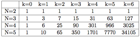
Here's are the values corresponding to the numerators:
A quick glance will show that each row is a multiple of N!. Simplifying to make the core structure more apparent yields the following table:
We have now narrowed down our original problem to understanding how each of these sequences is generated. All we need now that is to get the general formula of the terms in previous table, denoting it by S_N(k). We will then have:
The second row (for N=3) is easily identifiable as 2^(k+1)-1. The second column can be recognized as N(N-1)/2. Other than that, the underlying formula generating the other columns and rows is rather elusive. Again, please feel free to try for yourself!
For the remainder of the paper, we will refer to S_N(k) as the sequence for N. The sequence for N=4 therefore starts by 1, 6, 25, 90,...
My wife actually found another very nice relationship in the table. Denoting by En^k the elements in the table ((N-1)-th row and (k+1)-th column), we observe that:
See the 301 value? It's 3 * 90 + 31.
A very nice relationship, but unfortunately very difficult to exploit for our purpose!
(This is part 2 of a series of posts on iTunes randomness. The introduction and a link to all parts can be found here.)
Naïve approach: Take 1
Considering N songs , let's start with the most extreme case: what is the probability that each song will be heard once after N songs are played? That is to say k=0, and each song is played exactly once, without any songs being listened to twice. The sequences satisfying this are all the possible permutations of N songs, which is N!, while the number of possible song orderings is N^N, which gives us:
Another way to obtain the previous results is to make the following reasonning:
- the first song played has no impact on the probability
- the requirement for the second song is to be different from the first, which occurs with probability (N-1)/N
- the requirement for the third song is to be different from the first two, which occurs with probability (N-2)/N
- the requirement for the i-th song is to be different from the first i-1, which occurs with probability (N-i+1)/N
- the requirement for the last song is to be different from the first N-1, which occurs with probability 1/N
Putting all the pieces together also yields:
So let's look at the next case: with still N songs in our playlist, what is the probability that each song will be heard at least once after N+1 songs are played? In other words, what is the probability that k=1, and one, and only one, song will have been heard twice, and all others once? A possible scenario with 5 songs would be: 3-2-1-5-1-4.
So how many song orderings satisfy this scenario? It's a little trickier, but one way to look at the number of successful songs ordering is as follows:
- Out of the N songs, select the one that will be played last (N possibilities).
- Out of the remaining N-1 songs, select the one that will be played twice (N-1 possibilities).
- We now have N songs (N-1 unique, and one duplicate) that we need to order for the first N plays. There are N!/2 ways of doing so (dividing by 2 because two songs are identical).
- With N+1 songs being played, the size of the universe of song orders is now N^(N+1).
Putting the pieces together yields:
However, this approach does not generalize easily. Why? Consider N+2 plays, so k=2. We now have to distinguish two cases for the two extra plays: do they correspond to the same song or to different songs? Do we have 1-2-2-2-3 or 1-2-1-2-3? What about k=17? How do we split the additional 17 plays across the N songs? Although not impossible, it is a rather difficult task to determine all the ways of splitting the k extra plays across the N songs.
Naïve Approach: Take 2
Previously we looked at computing P(k|N) for fixed k to understand the relationship for small k and then derive a more general formula for any k. We can also take the opposite approach: compute P(k|N) for all k and small values of N, and see if we can generalize from there.
Consider 2 balls. What is P(k|2)? After hearing the first of the two songs, what is the probability of listening to it k more times before hearing the unheard song and ending the successful order of length k+2? We therefore derive:
For N=3, we get awfully close to the former brick wall. For instance, if k=7, we know that 7 songs will be repeats, but we don't know how the repeats will be spread out across the songs. Will it be 1-1-1-2-1-1-1-1-1-3 with 1 getting all the repeats, or something more balanced out like 1-2-1-2-2-1-1-1-2-3?
When I posted my predictions for the end of the season, I felt like I had some time before having to update these. However, in light of recent results, namely the Lakers pretty hot streak and a back-from-25-down comeback in New Orleans, the hype is back as to whether or not the Lakers will make it into the finals. Some have even argued that given how tight the last Playoff spots are in the West, the Lakers can even hope to get in the 7th or even 6th spot. But their future is not entirely in their hands, a lot depends on how the Warriors, Jazz and Rockets perform.
Let's see how the odds of each of these teams making it into the Playoffs has evolved and upadte our forecasts based on most recent games:

Only in Hollywood-land could an NBA team's probability of making the Playoffs jump from 10% to 40% in a matter of three weeks with only a quarter of the season remaining. All experts (and stats bloggers like me :-)) agreed that the Lakers' Playoff run would require a big slip by one or more of the team's ahead, and that is exactly what the Jazz is handing the Lakers on a silver.... scratch that, golden platter, with a probability drop from 90% to 55% over the same three weeks! Talk of a big slip! But to make this the perfect Hollywood script, the Lakers should clinch that 8th spot with a win on the final regular season against Houston...
Here's a table summarizing most recent values as of 2013-03-08:
| Team | Playoff Probability |
| SAS | 100% |
| OKC | 100% |
| LAC | 100% |
| MEM | 100% |
| DEN | 100% |
| GSW | 98.9% |
| HOU | 90% |
| UTA | 55.2% |
| LAL | 43% |
| POR | 7.3% |
| DAL | 5.6% |
| MIN | 0% |
| PHO | 0% |
| NOH | 0% |
| SAC | 0% |
Given the current excitement and hype, I'm guessing I will be posting updates sooner rather than later!
This recent article in French District (for French People in California) looks at how may people speak French in each of the US states. In order to do this, Facebook statistics are used, by looking at how many individuals in each state have listed French as a language. States are then ranked based on those absolute numbers. The main insights the author draws is that California has the most french speaking individuals (213,200) and Wyoming the least (1,440).
Personally, I don't find this super insightful and actually found the results to be presented in a misleading way.
There are definitely some questions we need to ask ourselves first before plunging into the data:
- Is the proportion of Facebook users in the population the same across states? The article answers this implicitly and hints that the proportion ranges at least from a half to two-thirds.
- Is the proportion of facebook users reporting their language the same across states? One could imagine that in more culturally diverse environments such as New York or California people might be more used to sharing this type of information.
- The article does sometimes put the absolute number of French speakers in perspective based on the state's population. Nonetheless, the ranking in the article is based on absolute numbers. So naturally we would expect California and Wyoming to have opposite values. Does that tell us anything?

Based on the values reported in the article I was able to rank states by proportion of reported French-speaking Facebook users in the population:
| State | % of French-Speaking Facebook Users |
| District of Columbia | 2.5% |
| New York | 0.9% |
| Nevada | 0.9% |
| Florida | 0.7% |
| Hawaii | 0.7% |
| California | 0.6% |
| Alaska | 0.5% |
| Illinois | 0.4% |
| Georgia | 0.4% |
| Louisiana | 0.4% |
| Texas | 0.3% |
| Pennsylvania | 0.3% |
| Ohio | 0.3% |
| New Jersey | 0.3% |
| Arizona | 0.3% |
| Wisconsin | 0.3% |
| Oregon | 0.3% |
| Montana | 0.3% |
| North Dakota | 0.3% |
| Wyoming | 0.3% |
| Oklahoma | 0.2% |
| Arkansas | 0.2% |
| Mississippi | 0.2% |
| South Dakota | 0.2% |
Although not perfect, this does provide a better comparison. District of Colmbia is mentioned in the original article as having the highest proportion, but nowhere does it state that this value is almost three times the value for the second highest state, New York. Definitely puts things into perspective!
And California despite having the largest absolute number is sandwiched between Hawaii and Alaska, probably not the states you would have thought of first!
Of course this ranking is only meaningful if we assume that the two previous assumptions hold on the proportions of Facebook users and language reporting are constant across states.
Oh and by the way, French people like referring to Facebook as "Face de Bouc" which sounds the same but literally means "billy goat face" :-)
(This is part 1 of a series of posts on iTunes randomness. The introduction and a link to all parts can be found here.)
Some definitions
Before jumping into the math, let's clearly define the terms and notations that will be used throughout the post(s).
Let N be the number of songs (all different) in our iTunes playlist.
Let p be the number of songs played in a sequence.
Let k=p-N. k will have an interesting interpretation later on and will be our parameter of interest.
A song order is any sequence of songs.
A song order of length p is any sequence of p songs.
A successful song order is a song order that satisfies our requirement that each song has been played at least once, and which stops as soon as this criteria has been met.
A successful song order of length p is a song order of length p that satisfies our requirement that each song has been played at least once, and the criteria is met when the p-th song is played.
P(p|N) is the probability that with N songs a successful song order will have length p. As mentioned previously, we will later switch to the notation P(k|N) = P(p-N|N) for ease of interpretation.
Example: Suppose we have N=4 songs.
A possible song order of length 7 is: 3-2-2-3-4-1-1. This particular song order is not a successful song order of length 7 as the criteria that each song has been played at least once is met when the 6-th song is played, the elusive song number 1.
A successful song order of length 7 would be: 4-1-1-4-2-1-3.
An obvious but important fact to notice is that in a successful song order of length p, we necessarily have p ≥ N. If we want to listen to N songs each at least once, at least N songs will need to be listened to! Recall that we defined k=p-N, so in successful song orders, k ≥ 0. k can also be interpreted as the number of times a song already listened to is repeated. Taking our previous example: 4-1-1-4-2-1-3, N=4, p=7, and so k=3, which accounts for the two times track 1 and the one time track 4 were re-listened to.
We are assuming that each pull is completely random, that is to say that each ball has an equal probability of 1/N to be pulled, even the one just pulled. Now this assumption is not exactly true in the iTunes world as discussed here, here and here, but is nonetheless a reasonable assumption for our problem.
Initial Plots
Some simple R code can generate music-listening simulations, random sampling songs until all have been heard at least once. For each number of song in the playlist ranging from 1 to 1000, 2000 simulations were performed to estimate the average number of total songs played to make the order successful. Results are presented in the following curve with red dots representing simulation results and the blue curve a fitted smooth line.
The curve is extremely smooth, and it very roughly seems like you need to hear about six times as many songs as you have in your playlist to get to listen to each song at least once! The curve hints at some convex curvature which indicates taht as the size of the playlist increases the factor might also increase.
Taking a closer look at the ratio of total songs played over total songs in the playlist, we observe a highly interesting pattern as shown in the next plot.
The curvature observed in the first curve is confirmed with the plot in the second curve, but what is most interesting is whether the ratio is bounded and will reach a final upper bound or whether it will continue to increase to infinity.
Another plot that we can look at but the analysis of which will not be covered in this paper is the distribution of plays for all the songs. In other words, once every song has been heard at least once, how many times has each song been played?
The distribution in the previous plot has some interesting characteristics. For any number of songs N, the minimum is always 1. This is because our song ordering ends when the last elusive song has been heard, so the last song played will have be heard once and only once. The mean and median are very close with the mean slightly higher. This observation makes sense given the distribution is lower-bounded by 1 but has no upper-bound (one song theoretically could be played any number of times before we obtain a successful song ordering). As for the median, the curve is actually the ratio we had observed in our second curve, always increasing but at slower rates and seeming to hover at around 6-7 when we reach 1000 songs in our playlist.
Reverting back to our original question of number of song plays required, the problem seems like a rather straightforward one at first (we have all done our share of blue and red ball pulling from urns at some point in a stat classe). If that is your feeling as well, we strongly urge you to attack the problem with the usual techniques, it will probably help better understand the approaches and mindset detailed in the rest of this paper.