NBA stock: 2016 is a highly volatile year!

Some things never change.

I haven't followed the new 2015-2016 NBA season as closely as I would have, but it's impossible to ignore that our two finalists from last years are still dominating their conferences, San Antonio keeps chugging along as it has always done since like forever, and similarly to last year the Lakers and 76ers are in for a terrible season if the first 20% of the season is any indication.

That being said, there is a rather lengthy list of surprises, good and bad:

• The Knicks were plain awful last year but now have a winning record
• The Rockets and Clippers gave us an intense Western Conference semifinals yesterday both playing at a very high level but both now have losing records
• The Hawks dominated the Eastern Conference last year yet are now ranked 6th in that same conference
• The Pelicans made the Playoffs last year but this year are playing just slightly better than the Lakers
• The Jazz were ranked 11th in the Western Conference last year, and are now ranked second

I could go on, but you get the idea. Now of course, nobody would expect every season to be an exact replicate of the previous one, players get injured, players transfer, coaches come and go... So some volatility in rankings is expected, but the question is how much?

Going back up to the 2005-2006 season, I pulled final regular season rankings for each season and each team (taking relocations into account for the Sonics, Bobcats and Hornets), and looked at absolute change from year to year. For instance, the Toronto Raptors finished 10th of the Eastern Conference in 2012-2013, 3rd in 2013-2014, 4th in 2014-2015. This would therefore be counted as a change of 7, followed by a change of 1 in conference ranking. Rank changes were averaged across all teams for each year. Here's the evolution of average rank change across all teams:

It appears that my hunch was not entirely unfounded: as of today (2015-11-24), current rankings have never been as different from the previous year going back to 2005-2006! (of course the season has only kicked off, and we are not entirely comparing apples to apples). 2014 was a close second, when 6 out of 30 teams had their conference rankings change by 7 or more positions.

What if we were to split out results for each conference?

It appears that the Eastern Conference is typically much more volatile than than its western counterpart. Up until 2014-2015, the Western Conference had never had an average rank change exceeding 3.2, a value that the Eastern Conference exceeded 5 times in the last 9 years! But comparing the first 15 games of the 2015-2016 season to last year's final standings, we have an average rank change of 4, tying the maximum value ever observed in either conference.

To finish off, it would be interesting to put these values in context and evaluate how much carry-over there is from one season to the next. Is an average of 3 or 4 rank changes per team high? or low? Our baseline would be a completely randomized basketball association where players are completely reshuffled from one year to the next and so each year's ranking is entirely random. I ran 100,000 simulations to see what the expected number of rank changes would be.

It turns out that a value of 4 is not particularly extreme: in our purely randomized world, about 15% of seasons would be less volatile rank-wise than what we are witnessing today!

I've spent quite some time running basketball analyses, from the number of expected runs and the incremental value of home court advantage to trying to forecast game outcomes based on team performance, yet it seems my conclusion is always the same: there is so much statistics can uncover, no matter what approach you take there always seems to be a strong unexplained random component which makes every team, every season, every championship so unique!

iTunes Randomness Part 5: The Tangled Equations

(This is part 5 of a series of posts on iTunes randomness. The introduction and a link to all parts can be found here.)

The tangled equations

Let's revisit our decomposition of 90:
1-1-1; 1-1-2; 1-1-3; 1-2-2; 1-2-3; 1-3-3; 2-2-2; 2-2-3; 2-3-3; 3-3-3.

Thinking back of our elevator metaphor, each of these numbers indicates time spent roaming around a given floor (listening to a previously heard song) and the number actually indicates on which floor the wandering is taking place. So 1-3-3 means you stayed an extra time period on level 1, and two on level 3.

All the paths are then the ways of wasting three time periods on three different floors. BUT, and this is a very important caveat, the numbers have to be in increasing order: 1-3-2 would not be an acceptable path. Indeed, the only ways of taking 3 items with replacement among 1, 2 and 3 with replacement and with numbers increasing are:

1-1-1, 1-1-2, 1-1-3, 1-2-2, 1-2-3, 1-3-3, 2-2-2, 2-2-3, 2-3-3, 3-3-3

Does this help us? Yes, because there is now another hidden recursion in the process!

We were here studying k=3, but what did the breakout look like at k=2? Let us list all the ways of taking 2 items with replacement among 1, 2 and 3 with replacement and with increasing numbers:

1-1, 1-2, 1-3, 2-2, 2-3, 3-3

It can be verified that the sum product here yields 25 which is the value in the second table of the sequences (part 3) for k=2 and N=4.

Based on this sequence for k=2, how can the sequence for k=3 be constructed?
If we look at all sequences starting with 1, then all k=2 sequences listed in red can be added to the right of the 1:

1-1-1, 1-1-2, 1-1-3, 1-2-2, 1-2-3, 1-3-3

If we now look at all sequences starting with 2, only the sequences for k=2 listed in red starting with 2 or 3 can be added as we cannot go back from 2 to 1, yielding:

2-2-2, 2-2-3, 2-3-3

Finally there is only one sequence listed in red starting with 3 that can be added to a 3:

3-3-3

This illustrates how the 10 sequences for k=3 listed at the top of this post can be generated from the k=2 sequences listed in red.

But remember that more than the sequences themselves it is their sum-product that we are interetsed in. Denoting by s_N^i (k) the sum product of all sequences starting with value i at time k for values ranging between 1 and N, then:

This looks a little confusing at first so let's illustrate the process with N=4 in the following figure:

Each column is a new "time point", and each row represents an s_N^i (k). Each arrow is color-coded according to the multiplication involved (times 1 for green, times 2 for orange and times 3 for blue). The last row is the sum of the s_N^i (k) at a given time-point, and – oh miracle! – the sum corresponds to the mysterious sequence observed in the table of our sequences in part 3 for N=4. Another fun fact to notice is that the sum is also the first row shifted by one, which makes sense as:

So now can we actually obtain the full explicit formula for the sequence itself. It involves some work as we unwind the tangled equations, working backwards from s_3^3 (k) to s_3^2 (k) to s_3^1 (k).

The calculations are a little lengthier for $s_3^2(k)$:

And finally:

No easy task, but we finally have our general formula generating the sequence for N=3:

The tangled equations can be used again for N=4:

More generally, we can start working our way backwards for the general case:

However, this has not allowed me to fully grasp the general formula for our sequence of interest s_N^1 (k) = S_N (k) for any N, which is the remaining piece of our puzzle.

An important observation can nonetheless be made. It seems as if the formula for s_1^k (N) is composed of all the integers 1 through N-1 to the power k+1:

The alpha_j coefficients also seem to alternate between positive and negative values.

Now what?

iTunes Randomness Part 3: Hidden Recursions

(This is part 3 of a series of posts on iTunes randomness. The introduction and a link to all parts can be found here.)

Recursion

From the past sections, it clearly appears as if the naïve approaches, despite potentially leading to the correct answer, would require much effort and are not the ideal path to proceed. Let us try to put off counting all possible permutations to later if possible.

Another way to think of the problem is to actually stop and think at what happens whenever a song is played. Only two things can happen: it is either a new song or one already heard.

More formally, denoting by Q(u, p) the probability of having heard u unique songs after p plays:

We can initialize by setting Q(1,1)=1 and Q(i,j)=0 if i>j.

When faced with such recursions, it is often helpful to expand back a few terms and try to see if a certain tendency or pattern emerges. You can try it out for yourself here, things get very messy very quickly with no clear trend in sight.

A little too early to shout victory, but at least we can write a nice recursive R function to quickly compute the P(k|N) probabilities, and no longer have to rely on simulations.

How are our P(k|N) related to the above Q(u,p) probabilities? Recall that P(k|N) is the probability of having listened to all N songs at least once after exactly p=N+k plays and not a song sooner! This means that after N+k-1 plays, we have heard all songs except one at least once, and on the next play we will hear the final elusive song (event that occurs with probability 1/N). Putting the pieces together:

First small victory!

The hidden sequences

Now that we have a way of getting exact probability values, is there any way we could get a glimpse of what the solution looks like?

For a given number of cards (2, 3, 4, ...) we have computed the P(k|N) probabilities. The numbers were quite ugly, but what really interests us is the numerator as the denominator will always be N^(N+k) which is the size of the universe for playing a random sequence of N songs N+k times (and this indeed what we saw when computing P(0|N), P(1|N) and P(k|2) in our first approaches.

Here's are the values corresponding to the numerators:

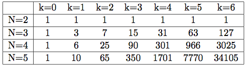
A quick glance will show that each row is a multiple of N!. Simplifying to make the core structure more apparent yields the following table:

We have now narrowed down our original problem to understanding how each of these sequences is generated. All we need now that is to get the general formula of the terms in previous table, denoting it by S_N(k). We will then have:

The second row (for N=3) is easily identifiable as 2^(k+1)-1. The second column can be recognized as N(N-1)/2. Other than that, the underlying formula generating the other columns and rows is rather elusive. Again, please feel free to try for yourself!

For the remainder of the paper, we will refer to S_N(k) as the sequence for N. The sequence for N=4 therefore starts by 1, 6, 25, 90,...

My wife actually found another very nice relationship in the table. Denoting by En^k the elements in the table ((N-1)-th row and (k+1)-th column), we observe that:

See the 301 value? It's 3 * 90 + 31.

A very nice relationship, but unfortunately very difficult to exploit for our purpose!

iTunes Randomness Part 2: Naïve Approaches

(This is part 2 of a series of posts on iTunes randomness. The introduction and a link to all parts can be found here.)

Naïve approach: Take 1

Considering N songs , let's start with the most extreme case: what is the probability that each song will be heard once after N songs are played? That is to say k=0, and each song is played exactly once, without any songs being listened to twice. The sequences satisfying this are all the possible permutations of N songs, which is N!, while the number of possible song orderings is N^N, which gives us:

Another way to obtain the previous results is to make the following reasonning:

• the first song played has no impact on the probability
• the requirement for the second song is to be different from the first, which occurs with probability (N-1)/N
• the requirement for the third song is to be different from the first two, which occurs with probability (N-2)/N
• the requirement for the i-th song is to be different from the first i-1, which occurs with probability (N-i+1)/N
• the requirement for the last song is to be different from the first N-1, which occurs with probability 1/N

Putting all the pieces together also yields:

So let's look at the next case: with still N songs in our playlist, what is the probability that each song will be heard at least once after N+1 songs are played? In other words, what is the probability that k=1, and one, and only one, song will have been heard twice, and all others once? A possible scenario with 5 songs would be: 3-2-1-5-1-4.
So how many song orderings satisfy this scenario? It's a little trickier, but one way to look at the number of successful songs ordering is as follows:

• Out of the N songs, select the one that will be played last (N possibilities).
• Out of the remaining N-1 songs, select the one that will be played twice (N-1 possibilities).
• We now have N songs (N-1 unique, and one duplicate) that we need to order for the first N plays. There are N!/2 ways of doing so (dividing by 2 because two songs are identical).
• With N+1 songs being played, the size of the universe of song orders is now N^(N+1).

Putting the pieces together yields:

However, this approach does not generalize easily. Why? Consider N+2 plays, so k=2. We now have to distinguish two cases for the two extra plays: do they correspond to the same song or to different songs? Do we have 1-2-2-2-3 or 1-2-1-2-3? What about k=17? How do we split the additional 17 plays across the N songs? Although not impossible, it is a rather difficult task to determine all the ways of splitting the k extra plays across the N songs.



Naïve Approach: Take 2

Previously we looked at computing P(k|N) for fixed k to understand the relationship for small k and then derive a more general formula for any k. We can also take the opposite approach: compute P(k|N) for all k and small values of N, and see if we can generalize from there.

Consider 2 balls. What is P(k|2)? After hearing the first of the two songs, what is the probability of listening to it k more times before hearing the unheard song and ending the successful order of length k+2? We therefore derive:

For N=3, we get awfully close to the former brick wall. For instance, if k=7, we know that 7 songs will be repeats, but we don't know how the repeats will be spread out across the songs. Will it be 1-1-1-2-1-1-1-1-1-3 with 1 getting all the repeats, or something more balanced out like 1-2-1-2-2-1-1-1-2-3?

iTunes Randomness Part 1: Initial Plots

(This is part 1 of a series of posts on iTunes randomness. The introduction and a link to all parts can be found here.)

Some definitions

Before jumping into the math, let's clearly define the terms and notations that will be used throughout the post(s).

Let N be the number of songs (all different) in our iTunes playlist.

Let p be the number of songs played in a sequence.

Let k=p-N. k will have an interesting interpretation later on and will be our parameter of interest.

A song order is any sequence of songs.

A song order of length p is any sequence of p songs.

A successful song order is a song order that satisfies our requirement that each song has been played at least once, and which stops as soon as this criteria has been met.

A successful song order of length p is a song order of length p that satisfies our requirement that each song has been played at least once, and the criteria is met when the p-th song is played.

P(p|N) is the probability that with N songs a successful song order will have length p. As mentioned previously, we will later switch to the notation P(k|N) = P(p-N|N) for ease of interpretation.

Example: Suppose we have N=4 songs.
A possible song order of length 7 is: 3-2-2-3-4-1-1. This particular song order is not a successful song order of length 7 as the criteria that each song has been played at least once is met when the 6-th song is played, the elusive song number 1.
A successful song order of length 7 would be: 4-1-1-4-2-1-3.

An obvious but important fact to notice is that in a successful song order of length p, we necessarily have p ≥ N. If we want to listen to N songs each at least once, at least N songs will need to be listened to! Recall that we defined k=p-N, so in successful song orders, k ≥ 0. k can also be interpreted as the number of times a song already listened to is repeated. Taking our previous example: 4-1-1-4-2-1-3, N=4, p=7, and so k=3, which accounts for the two times track 1 and the one time track 4 were re-listened to.

We are assuming that each pull is completely random, that is to say that each ball has an equal probability of 1/N to be pulled, even the one just pulled. Now this assumption is not exactly true in the iTunes world as discussed here, here and here, but is nonetheless a reasonable assumption for our problem.


Initial Plots

Some simple R code can generate music-listening simulations, random sampling songs until all have been heard at least once. For each number of song in the playlist ranging from 1 to 1000, 2000 simulations were performed to estimate the average number of total songs played to make the order successful. Results are presented in the following curve with red dots representing simulation results and the blue curve a fitted smooth line.

The curve is extremely smooth, and it very roughly seems like you need to hear about six times as many songs as you have in your playlist to get to listen to each song at least once! The curve hints at some convex curvature which indicates taht as the size of the playlist increases the factor might also increase.

Taking a closer look at the ratio of total songs played over total songs in the playlist, we observe a highly interesting pattern as shown in the next plot.

The curvature observed in the first curve is confirmed with the plot in the second curve, but what is most interesting is whether the ratio is bounded and will reach a final upper bound or whether it will continue to increase to infinity.

Another plot that we can look at but the analysis of which will not be covered in this paper is the distribution of plays for all the songs. In other words, once every song has been heard at least once, how many times has each song been played?

The distribution in the previous plot has some interesting characteristics. For any number of songs N, the minimum is always 1. This is because our song ordering ends when the last elusive song has been heard, so the last song played will have be heard once and only once. The mean and median are very close with the mean slightly higher. This observation makes sense given the distribution is lower-bounded by 1 but has no upper-bound (one song theoretically could be played any number of times before we obtain a successful song ordering). As for the median, the curve is actually the ratio we had observed in our second curve, always increasing but at slower rates and seeming to hover at around 6-7 when we reach 1000 songs in our playlist.

Reverting back to our original question of number of song plays required, the problem seems like a rather straightforward one at first (we have all done our share of blue and red ball pulling from urns at some point in a stat classe). If that is your feeling as well, we strongly urge you to attack the problem with the usual techniques, it will probably help better understand the approaches and mindset detailed in the rest of this paper.

iTunes and Shuffling: The unintended consequences of perfect randomness

Wait, haven't I already heard this song?

You're at your desk playing a game, coding, writing emails, checking whether your Facebook friends are as bored as you, checking the latest basketball results – or better yet – checking Statisticator's blog to look at basketball results predictions.

And then it happens.

The iTunes song that is playing right now. You've already heard yesterday, and maybe even the day before. You check iTunes and indeed it already has multiple plays whereas there are a whole bunch of other songs that have never been played.

How is that possible?

More questions then sprout: how many songs will I listen to before hearing each of the songs in my playlist at least once? Once I have heard each song at least once, how many times will I have listened to the song with maximum plays?

To make a more common statistical analogy, suppose you have an urn with N balls each uniquely numbered 1 through N. You then proceed to pull a ball, take note of its number (kind of like bingo), and then place it back in the urn. The question is then: how many balls will you have to pull in order to reach a point where you will have pulled each of the N different balls at least once?

Before jumping into the theory, a few words should be said about how shuffling works in iTunes, and what other iTunes-related analyses have reported.

There are two types of shuffling options in iTunes (at least used to be before version 11): "shuffle" and "party shuffle". With "shuffle" iTunes will randomly play all the songs in your library \textit{without} replacement. It simply creates a random permutation of your songs, and all songs will be played once and only once. This feature does not interest us in the framework of this paper. The other option, "party shuffle", randomly plays songs \textit{with} replacement. This is the feature that interests us: after any given song has been played, any song (including the one just finished) has an equal probability of being played. Steve Jobs has often emphatically declared that the shuffling in both cases was entirely random, which we will use as our key assumption.

While not the primary purpose of this paper, it is worthwhile to mention that there are numerous discussions on iTunes' randomness on the Internet. Certain users have noted that the same sequence of four or five songs is always played in the exact same order, suggesting the permutation is not perfect and the algorithm relies on some faulty pseudo-randomness. Others comment that the algorithm incorporates user star rating to determine the order in which to play the songs with a tendancy of playing five-starred songs more. Another analysis suggests that not all songs are created equally, observing that popular songs and artists, as well as songs purchased from the iTunes store, are played more often than expected.

Again, our purpose here is not to explore iTunes' randomness (or for that matter the randomness of any other shuffling mode on other devices), but to determine some of the consequences of the assumed perfect randomness on the number of times we will need to play songs before all of them are heard.

Perhaps perfect randomness is not such a desirable feature after all!

We will tackle these questions through different posts:

• Part 1 will contain some initial plots, as well as definitions and notations used in further parts
• Part 2 will tackle the problem using some more naive methods
• Part 3 will look at the elegant hidden recursions involved in the problem
• Part 4 is the One-Way Elevator theory generating the recursions in Part 3
• Part 5 will solve the Tangled Equations brought to light with the One-Way Elevator
• Part 6 will move one step beyond the Tangled Equations and attempt to solve them in a more general context with regression tools
• Part 7 will put all the pieces back together!