Tuesday Oct 29 2013: Bulls at Miami, who will win?

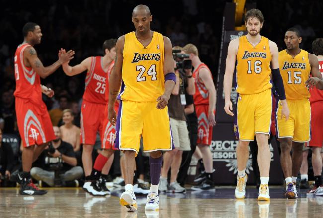
The 2013-2014 NBA season kicks-off Tuesday October 29th and the spotlight will be the return of two of the injured megastars: the Bulls' Derrick Rose in Miami, and the Kobe Bryant's Lakers host the Clippers.

On this blog we love drama, we love high intensity games, but we also like tough questions. Such as: who will win those two games? And while we're at it, who will come out victorious of the other 1228 games of the season?

In this post I will present my efforts to predict the outcome of a game based on metrics related to the two opposing teams.

The data

The raw data consisted of all regular-season NBA games (no play-offs, no pre-season) since the 1999-2000 season. That’s right, we’re talking about 16774 games here. For each game I pulled information about the home team, the road team and who won the game.


The metrics

After pulling the raw data, the next step was to create all the metrics relate to the home and road team’s performance up until the game I want to predict the outcome of. Due to the important restructuring that can occur in a team over the off-season, each new season starts from scratch and no results carried over from one season to the next.

Simple Metrics
The simple metrics I pulled were essentially the home, road and total victory percentages for both the home team and the road team. Say the Dallas Mavericks, who have won 17 of their 25 home games and 12 of their 24 road games visit the Phoenix Suns who have won 12 of their 24 home games and 13 of their 24 road games, I would compute the following metrics:

• Dallas home win probability: 17 / 25 ~ 68.0%
• Dallas road win probability: 12 / 24 ~ 50.0%
• Dallas total win probability: 29 / 49 ~ 59.2%
• Phoenix home win probability: 12 / 24 ~ 50.0%
• Phoenix road win probability: 13 / 24 ~ 54.2%
• Phoenix total win probability: 25 / 48 ~ 52.1%

Discounted simple metrics
However, these statistics seemed a little too simplistic. A lot can happen in the course of a season. Stars can get injured or return from a long injury. A new team might struggle at first to play with each other before really hitting their stride. So I included some new metrics which have some time discounting. A win early in the season shouldn’t weigh as heavily as one in the previous game. In the non-discounted world we kept track, for home games and road games separately, of the number of wins and number of losses, incrementing one or the other by 1 depending on whether the team won or lost. We do exactly the same here with a discount factor:

new_winning_performance = discount_factor * old_winning_performance + new_game_result

new_game_result is 1 if they won the game, 0 if they lost.

When setting the discount factor to 1 (no discounting), we are actually counting the number of wins and are back in the simple metrics framework.

To view the impact of discounting, let us walk through an example:
Let’s assume a team won it’s first 3 games then lost the following 3, and let us apply a discount factor of 0.9.

• After winning the first game, the team’s performance is 1 (0 * 0.9 + 1)
• After winning the second game, the team’s performance is 1.9 (1 * 0.9 + 1)
• After winning the third game, the team’s performance is 2.71 (1.9 * 0.9 + 1)
• After losing the fourth game, the team’s performance is 2.44 (2.71 * 0.9 + 0)
• After losing the fifth game, the team’s performance is 2.20 (2.44 * 0.9 + 0)
• After losing the sixth game, the team’s performance is 1.98 (2.20 * 0.9 + 0)

But now consider a team who lost their first three games before winning the next three:

• After losing the first game, the team’s performance is 0 (0 * 0.9 + 0)
• After losing the second game, the team’s performance is 0 (0 * 0.9 + 0)
• After losing the third game, the team’s performance is 0 (0 * 0.9 + 0)
• After winning the fourth game, the team’s performance is 1 (0 * 0.9 + 1)
• After winning the fifth game, the team’s performance is 1.9 (1 * 0.9 + 1)
• After winning the sixth game, the team’s performance is 2.71 (1.9 * 0.9 + 1)

Although both teams are 3-3, the sequence of wins/losses now matters. A team might start winning more if a big star is returning after an injury of due to a coach change or some other reason so our metrics should reflect important trend changes such as those. Unsure of what the discounting factor should be, I computed the metrics for various values.

Discounted opponent-adjusted metrics
A third type of metric I explored was one where the strength of the opponent is incorporated to compute a team’s current performance. In the above calculations, a win was counted as 1 and a loss as 0, no matter the opponent. But why should that be? Just like in chess with the ELO algorithm, couldn’t we give more credit to a team beating a really tough opponent (like the Bulls snapping the Heat’s 27 consecutive wins), and be harsher when losing to a really weak team?
These new metrics were computed the same way as previously (with a discounting factor) but using the opponent’s performance instead of 0/1.

Let’s look at an example. The Thunder are playing at home against the Kings. The Thunder (pretty good team) have a current home win performance of 5.7 and a current home loss performance of 2.3. This leads to a “home win percentage” of 5.7 / (5.7 + 2.3) = 71%. The Kings (pretty bad team) have a current road win performance of 1.9 and a current road loss performance of 6.1. This leads to a “road win percentage” of 1.9 / (1.9 + 6.1) = 24%.

If the Thunder win:

• The Thunder’s home win performance is now: 0.9 * 5.7 + 0.24 = 5.37
• The King’s road loss performance is now: 0.9 * 6.1 + (1 - 0.71) = 5.78

If the Thunder lose:

• The Thunder’s home loss performance is now: 0.9 * 2.3 + (1 - 0.24) = 2.83
• The King’s road loss performance is now: 0.9 * 1.9 + 0.71 = 2.42

If you win, you get credit based off of your opponent’s win percentage. If you lose, you get penalized according to your opponent’s losing percentage (hence the 1- in the above formulas). The worst teams hurt you most if you lose to them.
As seen from the example between a very good team and a very bad one, winning does not guarantee that your win performance will increase and losing does not guarantee your losing performance will increase. The purpose is not to have a strictly increasing function if you win, it is to get, at a given point in time, an up-to-date indicator of a team’s home and road performance.


The models

For all the models, the training data was all games except those of the most recent 2012-2103 season which we will use to benchmark our models.

Very simple models were first used: how about always picking the home team to win? Or the team with the best record? Or compare the home team’s home percentage to the road team’s road percentage?

I then looked into logistic models in an attempt to link all the above-mentioned metrics to our outcome of interest: “did the home team win the game?”. Logistic models are commonly used to look at binomial 0/1 outcomes.

I then looked into machine learning methods, starting with Classification and regression trees (CART). Without going into the details, a decision tree will try to link the regressor variables to the outcome variable by a succession of if/else statements. For instance, I might have tracked over a two week vacation period whether my children decided to play outside or not in the afternoon, and also kept note of the weather conditions (sky, temperature, humidity,...). The resulting tree might look something like:

If it rains without wind tomorrow, I would therefore expect them to be outside again!

Finally, I also used random forest models. For those not familiar with random forests, the statistical joke behind it is that it is simply composed of a whole bunch of decision trees. Multiple trees like the one above are “grown”. To make a prediction for a set of values (rain, no wind), I would look at the outcome predicted by each tree (play, play, no play, play….) and pick the most frequent prediction.

The results

As mentioned previously, the models established were then put to the test on the 2012-2013 NBA season.

As most of the models outlines above use metrics that require some historical data, I can’t predict the first game of the season not having any observations for past games for the two teams (yes, I do realize that the title of the post was a little misleading :-) ). I only included games for which I had at least 10 observations of home games for the home team and 10 road games for the road team.

Home team
Let’s start with the very naive approach of always going for the home team. If you had used this approach in 2013, you would have correctly guessed 60.9% of all games.

Best overall percentage
How about going with the team with the best absolute record? We get a bump to 66.3% of all games correctly predicted in 2013.

Home percentage VS Road percentage
How about comparing the home team’s home percentage with the road team’s road percentage? 65.3% of games are correctly guessed this way. Quite surprisingly, this method provides a worse result than simply comparing overall records.

Logistic regressions
Many different models were tested here but I won’t detail each. Correct guesses range from 61.0% to 66.6%. The best performing model was the simplest one which only included the intercept and the overall winning percentage for the home team and the road team. The inclusion of the intercept explains the minor improvement to the 66.3% observed in the “Best overall percentage” section.
Very surprisingly, deriving sophisticated metrics discounting old performances in order to get more accurate readings on a team’s performance did not prove to be predictive.

Decision tree
Results with a decision tree was in the neighborhood of the logistic regression models, with a value of 65.8%.

Interestingly, the final model only looks at two variables and splits: whether the home team's home performance percentage (adjusted with a discounting factor of 0.5) is greater than 0.5 or not, and whether the road team's performance incorporating opponent strength (discounting factor of 1, so no discounting actually) is greater than 0.25 or not.

Random Forests
All our hopes reside in the Random Forests to obtain a significant improvement in predictive power. Unfortunately we obtain a 66.2% value, right where we were with the decision tree, the regression model and more shamefully the model comparing the two teams overall Win-Loss record!
When looking at which variables were most important, home team and road team overall percentages came up in the first two positions.


Conclusions

The results are slightly disappointing from a statistical point of view. From the simplest to the most advanced techniques, none are able to break the 70% threshold of correct predictions. I will want to revisit the analyses and try to break the bar. It is rather surprising to see how overall standings matter compared to metrics that are more time sensitive. The idea that the first few games of the season matter to predict the last few games of the season is a great insight. This can be interpreted by the fact that good teams will eventually lose a few consecutive games in a row, even against bad teams, but that should not be taken too seriously. Same with bad teams winning a few games against good teams, they remain bad teams intrinsically.

From an NBA fan perspective, the results are beautiful. It shows you why this game is so addictive and generates so much emotion and tension. Even when great teams face terrible opponents, no win is guaranteed. Upsets are extremely common and every game can potentially become one for the ages!

Who will make the Playoffs?

The All-Star weekend is a nice break in the middle of the regular season. Dunk contest, three-point contest, rising stars game and naturally the All Star game itself. A good break indeed from the intense regular season schedule.

But for me it offered a unique opportunity: no games for four consecutive nights! The perfect opportunity to run simulations. Many simulations.

A. Downpour. Of. Simulations.

You be the judge: the outcome of over 2 BILLION games were simulated.

I previously worked on some code to forecast the outcome of the rest of the season based on each team's latest performance, code which I have already used to look at the Lakers probability of making the Playoffs, and whether Dallas or LA (Lakers) had a better chance of making the Playoffs. But I was eagerly waiting for the All Star weekend to run the code for all days starting on December 1st 2012, in order to look at the trends and shifts in each team's probability of making the Playoffs, and each team's expected final standing.

Here are the results by conference.

Eastern Conference

Let's start by looking at the evolution of team standings:

And now for the evolution of the probability of making it to the Playoffs:

The last values as of February 15th 2013 give the following values:

Team	Position	Playoff Probability
MIA	1.196	100%
NYK	3.157	100%
BRK	4.455	99.8%
IND	4.076	99.8%
CHI	4.445	99.7%
ATL	4.942	99.6%
BOS	6.706	95.4%
MIL	7.230	91.4%
PHI	9.666	8.2%
TOR	10.195	4.2%
DET	10.588	1.8%
WAS	13.069	0.1%
CHA	14.470	0%
CLE	12.564	0%
ORL	13.241	0%

Although Philadelphia still has a glimmer of hope of making the Playoffs provided Milwaukee runs into a very bad stretch, the eastern teams making the Playoffs seem decided. The huge uncertainty however lies around positions 3-6 where all teams are extremely close. With the Brooklyn Nets facing Chicago and Indiana in the last two weeks of the regular season, the eastern final brackets will not be decided until the very end.


Western Conference

Similarly to what we did for the Eastern Conference, let's start by looking at the standings evolution:

And now for the "Playoff Probability" evolution:

The last values as of February 15th 2013 give the following values:

Team	Position	Playoff Probability
LAC	2.749	100%
OKC	2.371	100%
SAS	1.329	100%
DEN	4.899	99.9%
MEM	4.682	99.5%
GSW	5.824	97.5%
UTA	7.190	86.9%
HOU	7.550	80.7%
POR	9.752	14.8%
LAL	9.877	12.1%
DAL	10.376	8.1%
MIN	12.519	0.4%
NOH	12.870	0.1%
PHO	14.224	0%
SAC	13.788	0%

The story is a little different on the western front, where suspense is not around the center 3-6 positions and the final Playoff bracket but on the final eight spot. Houston has a good chance of keeping that spot which it currently holds, but Portland and Los Angeles (Lakers of course!) are on their heels from a safe-but-not-THAT-safe distance. Any slip and the two will pounce on the position!

I will provide updated probabilities as the season progresses!

From "Will they be champs?" to "Will they make the playoffs?"

I have not posted any basketball-related articles since sharing my data-driven predictions for the 2012 NBA Finals (unfortunately for me, the data suggested the Oklahoma City Thunder had a slight advantage against the Miami Heat).

But there has been SO much talk recently on the Los Angeles Lakers' performance that I just had to take a stab at predicting their season outcome.


Background

For those of you not too familiar with the situation, it has all the drama of a Hollywood script, and I will briefly summarize the situation.

The Lakers have had great results in the past years, winning the championship in 2009 and 2010, and being tough opponents in the other years. Over the 2012 summer and a disappointing 2012 year, they signed a couple of superstars: Steve Nash from Phoenix, desperate to win a championship and one of the league's top point guards, as well as Dwight Howard from Orlando, who can be quite a beast under the basket. On paper they were an All-Star team, nobody contested that. Almost everyone had them reaching the Finals, the only question was whether they would beat Miami or not.

But their performance so far surprised even the most pessimistic: they started the season by accumulating losses, and have lost more games than they have won since the start of the season. Things get worse as they are in the Western Conference which is much more competitive than the Eastern conference. Add in a fired coach, a surprising replacement coach, and you have all the drama necessary for a lot of ink to be poured!

Total confusion on the court has been a common sight in the Staples Center:

And so the questio has become: will the Lakers even make it to the NBA playoffs? Only the best eight teams of the Western conference make the playoffs. Many analysts have looked at historical data, noticing that the eight team in the West has an average of 48 wins, and if the Lakers want to reach 48 wins this season they need to start winning fast.

I've decided to take a slightly different approach, by tring to forecast what the rest of the season would look like for all teams based on the first half of the season. Also, the previous methodology ignores what the rest of the teams are doing in your conference, as well as the impact of playing another team also fighting for a playoff spot. When you win against one of those teams, it basically counts double!


Methodology

Here's the methodology I've taken:

• extract all of the 2012-2013 season scores and schedule data for all teams, namely home and away winning percentages
• for all upcoming games I compute the home team's probability of victory as follows:
  home team winning percentage / (home team winning percentage + away team winning percentage).
  For example: Let us say that Chicago with a 12-5 road record (70.8% road winning percentage) is visiting Miami with a 16-3 home record (84.2% home winning percentage), I would estimate Miami's probability of winning the game as:
  84.2% / (84.2% + 70.8%) = 54.4%.
• Based on this probability, I simulate the game's outcome and then update Chicago's and Miami's records (if Chicago wins, their road record is now 13-5 and Miami's home record becomes 16-4).
• I continue proceeding that way until all the season's games have been simulated. This then becomes one possible outcome for the season.
• I then repeat the entire process outlined above thousands of time to get an idea of all the scenarios that can play out.

Based on the simulations, I can then determine which teams are most likely to have the best record in the NBA, and, going back to our original question, how likely the Lakers are to make the playoffs.


Results

Here are the results (based on scores up to 21/01/2013):

Top three NBA records:

• First place:
  Oklahoma City Thunder (32.9%), San Antonio Spurs (29.2%), Los Angeles Clippers (28%)
• Second place:
  San Antonio Spurs (26.6%), Oklahoma City Thunder (24%), Los Angeles Clippers (23.4%)
• Third place:
  San Antonio Spurs (18.7%), Oklahoma City Thunder (17.6%), Los Angeles Clippers (17.1%)

Clearly, the odds are that these three teams will enter the playoffs with the best records and so most likely a Western Conference team will have homecourt advantage in the Finals!

As for the Lakers, here are the probabilities of their final standing in the Western conference:

Position	Probability
6	0.4
7	1.4
8	4.1
9	8.9
10	12.6
11	18.1
12	24.2
13	16.9
14	10
15	3.4

Wow! Only a 5.9% probability of the Lakers making the Playoffs!

But let's still monitor them closely, and I'll update these results in the weeks to come.

Please leave a comment if you have any questions/suggestions on the methodology and/or results!

  

The Dark Night Released

Today I wanted to take a closer look at the evolution of a movie's metrics around its release time. Do ratings go up, down? How long does it take for the ratings to stabilize? What about a movie's metascore (aggregated score from www.metacritic.com based on "official" critics)?

To kick this off, I looked at three movies for which I had sufficient data: Ice Age 3, Savages and the Dark Knight Rises. I was also interested in the Dark Knight Rises to see if the events surrounding the Aurora shooting had any impact.

Ice Age 3: Continental Drift

For this move the number of voters really jumped the week after the release (dashed vertical line).

As for the rating it dropped from a 7.1 pre-release "hype" to stabilize itself at 6.9. Interesting to see how quickly it stabilized (aside from the mini bump the second week, the rating of 6.9 was achieved the same weekend the movie was released).

Metascore followed a similar evolution with a sharp decrease right around release date. The stabilization in rating makes more sense as not many magazines and newspapers review the movie after its release.

Savages

Unfortunately I was not able to gather any pre-release data for this movie, but interesting to see again that the biggest jump in IMDB voters occurred two weeks after release.

Again, the rating very quickly stabilized a few days after release to 6.8.

 The metascore dropped fairly late although only by one point.

The Dark Knight Rises

 Despite trying to pull IMDB data up to two weeks in advance I was not able to collect any pre-release data for the third installment of the Dark Knight series.

Ratings dropped steadily from 9.2 to 8.9 over two weeks, again suggesting a fairly quick stabilization, especially as the number of voters increases.

The metascore had a sharp dropoff right around the release date, and the shooting, although it is unclear if there is any type of relation. Based on our very limited sample size it seems that metascore and rating always tend to drop around the release.

I am currently pulling more data for these movies and 15 others, so come back to check updated and new results. I will also try a meta-analysis to see if there is some common pattern in the evolution of the metrics across all movies.

Thunder VS Heat: Stormy match-up

Now that the final two final contenders, it's time for the final predictions of the 2012 NBA season!

On Sekou Smith's Hang Time Blog the experts favor Oklahoma City 5 votes to 1, but what do the stats say?

The same model that was used to correctly predict the Thunder in 5 against the Lakers, and had slightly favored the Spurs in 7 over the Thunder in 6, gives a small advantage to OKC given its track record and homecourt advantage, but the margin is extremely close:

Winner	Num games	Probability
OKC	4	6.4%
MIA	4	6.0%
OKC	5	13.8%
MIA	5	11.3%
OKC	6	15.0%
MIA	6	16.3%
OKC	7	17.0%
MIA	7	14.4%

So if I had to put my money down, it would be for the Thunder in 7 as 3 NBA.com experts claimed.
But be careful, Miami in 6 is a very close possibility!

NBA: Spurs VS Thunder

Time for a playoff update now that the two contenders for the Western Finals are known.

Everybody wants to see Spurs VS Heat, but before then comes the Thunder hurdle, and despite the Spurs impressive performance up til now, this is definitely going to be a tough challenge.

The method is exactly the same from my previous post (which correctly identified Thunder beating the Lakers in 5 as the most likely scenario!). Entering the last numbers in the model, here's what came out:

Probability of Spurs winning the series: 55.6%

Series breakout:

Winner	Number of games	Probability
Spurs	4	6.6%
Thunder	4	5.3%
Spurs	5	15.8%
Thunder	5	9.5%
Spurs	6	14.3%
Thunder	6	16.9%
Spurs	7	19.0%
Thunder	7	12.7%

The three most likely scenarios are:
Spurs in 7 (19.0%), Thunder in 6 (16.9%) and Spurs in 5 (15.8%).

For the overall playoffs, the latest numbers suggests the West as championship favorites for now:

NBA team	Champion Probability
SAS	34.4%
OKC	25.7%
MIA	21%
BOS	12%
IND	4.6%
PHI	2.4%

Verdict in the upcoming weeks!

Lakers - Thunder Series

This post is actually an expanded comment to Sekou Smith's Hang Time Blog on nba.com concerning the Lakers - Thunder series.

This series is one everybody has been waiting for since the start of the season.

Experience VS youth.
Kobe VS Kevin.

VS

A blowout in game 1.
An incredible comeback in game 2.

What's in store for the next 2 + X games?

5 nba.com's experts on Sekou's blog give their predictions after 2 games: one says 4, two say 5, and 2 say 6.

But what do the stats say?

I recently updated my model from the last two posts (here and here) in two ways: homecourt advantage is now incorporated (another post soon on this topic, namely how we can quantify it, whether all teams have a significantly higher probability of winning at home than on the road, and which teams have the greatest delta in home ganes vs away games), and by providing more details on each series with not only the probability of one team winning it but also the breakout in how many games the series will play out.

Which is exactly what I did here for the Lakers - Thunder series.

And now for the results:

Winner	Number of games	Probability
Thunder	4	22.2%
Thunder	5	30.4%
Lakers	6	5.8%
Thunder	6	17.2%
Lakers	7	9.5%
Thunder	7	14.9%

So Thunder in 5 is actually the most likely scenario, followed by Thunder in 4 and in 6. Overall, if you're a Laker fan you should feel depressed with Lakers having only a 15.3% probability of facing the Spurs. But I have to admit that I haven't factored Kobe-back-against-the-wall variable in my models :-)

Let me know your thoughts!

2012 NBA Playoffs: Updated forecasts

What a first round this has been!

Things were rather quickly expedited in the East, including the surprising elimination of the #1 team Chicago Bulls, surprising until we saw the following video at least:

Meanwhile, the West was really the wild wild west and gave us some thrilling comebacks and two stressful game sevens.

Chicago was the favorite to win the Championship after the first two games of the playoffs with an estimated probability of victory of 17.9%. Its elimination has freed up some room but for whom?

Oklahoma City, San Antonio and Miami were the runner ups, and while the names of the next three teams hasn't changed, their order has:

NBA team	Champion Probability
MIA	21.5%
OKC	21.2%
SAS	19.3%
BOS	10.2%
LAC	7.9%
IND	7.3%
PHI	6.6%
LAL	6%

However the results are slightly biased as of now in the sense that Miami and Oklahoma won their round 2 opener whereas San Antonio still hasn't played Game 1 against the Clippers. If it were to win, it would jump right back to the first spot with a probability of 24.6% of clinching the Larry O'Brien trophy, more than 3 percentage points ahead of Miami and Oklahoma City.

More updates at the end of round 2!

The Johnny Depp / Tim Burton collaboration

I don't think anybody could have remained oblivious to the new Dark Shadows movie coming out:

Yet another Johnny Depp / Tim Burton collaboration, it seems those two have been in the movie business forever ! Edward Scissorhands, Sleeph Hollow, Charlie and the Chocolate Factory, Alice in Wonderland, now this !

So this begs the question: why? What do I mean "why"? Well, do the two just really like working together, or have they both determined that their partnership was mutually beneficial in terms of the quality of the movies created together?

I pulled IMDB data for Johnny Depp and Tim Burton separately focusing only on Johnny Depp as an actor and Tim Burton as a director (did you know he was in the list of actors for M.I.B. 3 ???), and labelled the movies either as "Common movies, "Johnny Depp only" or "Tim Burton only".

Collaboration VS Solo

Here is a graph summarizing for each of the three categories the IMDB ranking of the movies:

The above plot in question is called a boxplot and is a quick way to compare sets of data. The dark bold horizontal line is the median, and the gray rectangles represent the 25%-50% interquantile range, meaning that only 25% of movies will have rating greater than the top of the rectangle, and only 25%

will have a value less than the bottom of the rectangle. The dashed lines (called "whiskers") give an idea of the spread of the most extreme values.

For instance, we see that the median value for "Common movies" is around 7.5, and the data is rather concentrated (no movie had a rating better than 8, and none worse than 6.5).

Now comparing to the movies Johnny and Tim did solo, we see that while their joint work did not produce their best-rated movies (8.2 with Platoon for Johnny, and 8.4 with Vincent for Tim), it definitely limited risks with no movies worse than 6.5, whereas at least 25% of the movies Johnny or Tim did by themselves got worse than 6.5.

What about gross revenue?

Another comment about the boxplot: the round circles represent 'outliers' in the sense that they are values way beyond the spread observed in the data.

For "Common Movies", the outlier is Alice in Wonderland which generated just over a billion dollars, despite being, ironically, their worst-rated movie together at 6.5!

For Johnny Depp, the data is quite interesting: all his solo movies seem to have generated less than 150 million dollars, except four which made 4 to 7 times that amount. No surprises here, all four are Pirates of the Caribbean. I'm sure Johnny Depp bank account is looking forward to the fifth installment!

As for Tim Burton, the movies he did with and without Johnny Depp have very similar profiles.

Ratings and box office revenue can be combined in a scatterplot:

On a side note, it is interesting to see from the above graph the relationship between IMDB rating and revenue for the Johnny-Tim collaboration (blue dots): the greater the revenue, the lower the rating!

Evolution over time

The natural follow-up question is how this collaboration fits with the historical trends for both Johnny Depp and Tim Burton.

In terms of ratings, the collaboration had a significant impact on movie quality for Johnny Depp at the beginning of his career but very little in recent years (which was what the earlier boxplots hinted at earlier), whereas the impact was essentially insignificant for Tim Burton (but it's interesting to notice that 5 of Tim Burton's last six were with Johnny Depp).

From a revenue perspective, the collaborative Alice in Wonderland generated as much as the Pirate of the Caribbean series for Johnny, whereas that same movie and Charlie and the Chocolate Factory were Tim Burton's two biggest revenue-generating movies.

Closing conclusions

If  were to summarize the previous findings in one sentence, it would be that Johnny Depp is currently repaying Tim Burton for having made him known in Hollywood early on his career with great-rated movies (Edward Scissorhands and Ed Wood) by starring in two huge hits (dollar-wise).

All this being said, it will be very interesting to see how well Dark Shadows performs and how it fits in with the current trends...

Dominion: Optimal "Big Money" strategy?

In a previous post I gave a quick overview of the rules of the board/card game Dominion.

Because there are so many different and attractive actions cards to purchase, they can be very tempting to purchase, especially those allowing you to draw and play even more action cards. However, a very simple yet efficient strategy at Dominion is called "Big Money" and essentially ignores all the action cards.

Big Money strategies

"Big Money" consists in only purchasing treasure cards and buying Provinces. Assuming a two-player game with 8 Provinces in play, I will look at how many turns it takes to buy 4 Provinces. As a hand consists of 5 cards and players only start with copper, the maximum hand value is 5, so before the first Province can be bought, silvers and golds will have to be bought.

The algorithm for "Big Money" can be written as:

• if hand value >= 8, buy Province
• otherwise, if hand value >= 6, buy gold
• otherwise, if hand value >= 3, buy silver
• otherwise, do nothing

But some variations exist. Indeed, in Dominion it is usually important to have a high money density, to maximise the value of a 5-hand card. So although coppers are worth 1 and cost nothing to buy, it would be foolish to gain as much of these as possible as the values of your hand will be capped at 5, and make higher purchases impossible. So going back to the variations, we ideally want as many gold as possible to raise the average value of a 5-card hand. But what about silvers? We need to buy at least one silver in order to buy a gold (4 coppers + 1 silver = 6, cost of a gold). But if the player has multiple turns with a hand of 3, 4 or 5, should silvers always be bought, or are they going to bring the average hand value down? Wouldn't it be worth skipping those turns and wait to buy gold instead?

I therefore created variations of Big Money, depending on variable k which is the maximum number of silvers the player will buy. If the player already has k silvers and has a turn with 3, 4 or 5 in money, the player will not buy a new silver:

• if hand value >= 8, buy Province
• otherwise, if hand value >= 6, buy gold
• otherwise, if hand value >= 3 and [less than k silvers in deck + hand + discard pile], buy silver
• otherwise, do nothing

Analysis results

And now for the long awaited results. Let us consider 9 different "Big Money" variants, respectively capping silvers at 1, 2, ...7, 8 and no capping, I've displayed the number of turns it took to buy 4 Provinces based, on 100,000 simulations in each case.

Apparently, capping is not a good idea, especially for very small values. For larger caps (7, 8), it is unlikely the limit will even be reached! But just to confirm let's take a closer look excluding the first two caps:

Looking at the mean number of turns in each situation:

• When Capping at 1 silver purchase, the average number of turns required to purchase 4 Provinces was 31.14.
• Capping at 2: 21.63 turns on average
• Capping at 3: 19.47  turns on average
• Capping at 4: 18.25  turns on average
• Capping at 5: 17.55  turns on average
• Capping at 6: 17.13  turns on average
• Capping at 7: 16.91  turns on average
• Capping at 8: 16.83  turns on average
• No capping: 16.80  turns on average

So, when applying "Big Money", don't think twice go ahead buy the most expensive treasure you can!

In the next post we will take a look at some characteristics of "Big Money". How much Gold will you end up with? How much money in total? On which turns can you expect to purchase your first three Provinces?

There is much literature about "big Money" and my objective is not to repeat what can easily be found elsewhere, but to use "Big Money" as a simple benchmark for other strategies I would like to model, explore and compare.

Who will be the 2012 NBA champs?

As of today, and after a shortened but game-packed season, the 2012 NBA playoffs are finally underway!

Let's take a look at the playoff bracket:

Some very interesting match-ups ahead!

But in addition to trying to catch as many games as possible, I also wanted to take a stab at predicting who would become the 2012 NBA champions of course!

Just as in the previous posts, I will start off with a very simple model and work from there to improve its reliability.

So, what simple model can be establish to predict the outcome of the match-up between two teams? Let's simply consider the number of victories they obtained during the course of the season and derive a probability of winning a game from there.

Let us assume team 1 won 50 games and team 2 won 40 games. I would then grossly estimate that team 1's probability of winning a game against team 2 is 50 / (50 + 44) ~ 56%.

Similarly to many other sports, each match-up is a best-of-seven, meaning that the first team to win 4 games gets to advance to the next round. Therefore, if team 1 has a probability p of winning a game against team 2, team 1's probability of winning the match-up is:

P(win match-up) = p⁴ (1 + 4 * (1 - p) + 10 * (1 - p)² + 20 * (1 - p)³)

Indeed, team 1 needs to win 4 games hence the p^4, and team 2 can win anywhere from 0 to 3 games with probability (1 - p). Depending on the number of games team 2 wins, the number of arrangements varies, yielding the 1, 4, 10 and 20. In the previous example, team 1 has an overall probability of winning the series of 62%, despite having won 25% more games during the season. This very simple framework can help explain the many upsets that are regularly witnessed.

So now that we can figure out the probability of team 1 winning its first match-up, we can go to the next step and figure out the probability that will win the series against the winner of the team 3 - team 4 match-up:

P(team 1 wins second round) = P(team 1 beats team 3) * P(team 3 beats team 4) + P(team 1 beats team 4) * P(team 4 beats team 3)

I started this script this morning when none of the games had been played yet, and obtained the following probabilities for each team of becoming the NBA champions:

NBA team	Champion Probability
CHI	15.0%
SAS	14.4%
OKC	11.3%
MIA	10.5%
IND	6.7%
LAL	5.8%
MEM	5.4%
ATL	5.0%
LAC	4.7%
BOS	4.3%
DEN	3.7%
ORL	3.3%
NYK	2.7%
DAL	2.6%
UTA	2.4%
PHI	2.2%

I re-ran the script after the results of today's first four games (good thing I'm single) and obtained the following similar results:

NBA team	Champion Probability
CHI	17.9%
OKC	14.1%
SAS	13.6%
MIA	13.0%
LAL	5.2%
MEM	5.0%
ORL	4.5%
ATL	4.4%
LAC	4.4%
IND	4.1%
BOS	3.8%
DEN	3.4%
UTA	2.2%
NYK	1.6%
DAL	1.5%
PHI	1.2%

Winning the first game did bump up the teams by a couple of percentage points, Oklahoma City now pulled in front of San Antonio.

But wait! Before you run to the closest sports betting bar to put down all your money on the Bulls, you should be aware that the current model doesn't account for certain external events such as... Derrick Rose tearing his ACL in the Bull's first game. The Bulls played great this year without Derrick in the lineup, but his absence is definitely going to hurt their chances...

Another surprise is the relatively low probabilities for the top teams of the season. Looking at the top 4 contenders, their cumulative probability of wining the title is barely over 50%. Again, this explains some of the regular surprises we see every now and again (every other year theoretically ;-) ).

There are many other caveats with this simple model, homecourt advantage is not taken into into account, nor is the fact that certain teams having already secured their playoff position rested their star players and lost games that were of no importance.

Nevertheless, I will try to continue improving the model and adress the current limitations. Naturally, I will also regularly post updated probabilities as the playoffs progress.

Now back to the replay of Kevin Durant's shot...

Predicting France's next president?

We're quite literally in the middle of the French Elections, a perfect opportunity to try to predict the new president 10 days ahead of time!

Before we jump in the model, a few words on the French system, thankfully much simpler than the US one!

French elections 101

The election is a two-step process. During the first step, called "first round" all candidates are eligible, and each french voter casts his vote for one of them.

After this first round, the two candidates having received the most votes go to the "second round" and are the only two eligible candidates at this point. This second round takes place exactly two weeks after the first round. Today we are right between the two rounds, and the two remaining candidates are current president Nicolas Sarkozy seeking his second term (left picture), and François Hollande (right picture).

 

The polls have been pretty much spot on predicting Nicolas and François would battle in the second round, with Francois Hollande having a slight advantage in first round votes.

So, can we predict who will win the second round?

I looked at historical results for the past six presidential elections (1974, 1981, 1988, 1995, 2002 and 2007), recording for each candidate first round and second round percentage of votes.

The model aims at computing the probability of becoming president for the candidate receiving the most votes in the first round.

Now out of the six past elections, the first round vote leader won only 3 elections with the challenger winning the other 3. So looking at the difference in first round percentage votes is not sufficient.

Based on various theories on election, it is also important to consider the percentage of votes received by other eliminated candidates with close affinities to the round-two candidates. Now with only 6 observations, it is difficult to introduce many variables, but I decided to add one more in addition to the first round delta percentage votes for the two leading candidates. This second variable is the delta between percentage votes for the candidates closest candidates. Let me explain based on an example:

Let us rank the 1995 first round candidates by left-right political affinity:

Candidate            First Round %       Sum closest two
Arlette Laguiller             5.30                  8.66
Robert Hue                    8.66                 28.60
Lionel Jospin                23.30                 11.98
Dominique Voynet              3.32                 41.87
Edouard Balladur             18.57                 24.16
Jacques Chirac               20.84                 23.31
Philippe de Villiers          4.74                 35.84
Jean-Marie Le Pen            15.00                  5.02
Jacques Cheminade             0.28                 15.00

For each candidate I then computed the sum of the two candidates immediately to the left and to the right on the political scale.

And the variable I introduce is the delta of this sum metric for the first round leader and the runner-up. So in 1995, te first round leader was Lionel Jospin, his first round percentage delta with second vote leader Jacques Chirac was 2.46 (23.30 - 20.84), and the "closest candidate delta" was -11.33 (11.98 - 23.31).

Model results

With these variables, I built a quick logistic model to estimate the probability of the first round leader to win the second round as a function of "first round delta" and "closest candidate delta".

Applying the model to the results of the 2012 first round results, indicates that the president for the next five years will be....

Nicolas Sarkozy !

Now, despite the small number of observations, I decided to exclude one of them which could be seen as an outlier. Indeed, in 2002 the extreme right party created a monumental surprise by reaching the second round. The second round became a right VS extreme right instead of the usual right VS left battle. And that year Jacques Chirac won the second round with an unprecedented 82% of votes whereas the values usually reside in the 45%-55% range.

Excluding that observation, the model was a perfect fit for the five remaining observations and predicted that the president for the next five years will be....

Nicolas Sarkozy !

Wait until May 6th to criticize...

Now, I could not agree more with the criticism the approach deserves of using the variables (including the intercept) in the model when we only have five or six observations.

But the objective here is not to publish in a stats journal, jsut to play around with the data. And all the polls indicate the François Hollande will be the next president. So in 10 days we'll see if this method that predicts Nicolas Sarkozy isn't as faulty as it would initially appear...